Introduction

This guide is designed to be the final workshop in the Basic HEC-HMS class. The goal is to develop a simple hydrologic model and calibrate the model to observed streamflow using gridded precipitation. Lectures and workshops from the Basic HEC-HMS class touch on components needed to create a hydrologic model. This guide ties everything together and gives you an opportunity to complete all the basic steps for a single application. This guide should take you approximately four hours to complete if you are new to HEC-HMS and hydrologic modeling. This guide is broken up into the following steps:

Download Streamflow Data
Delineate Modeling Elements Using HEC-HMS GIS Tools
Parameterize the Subbasin Element
Add Streamflow and Precipitation Data to the Project
Calibrate the Model
Document Final Model Parameters

Project Files

Download the initial files here:

Precipitation.zipGIS.zip

Background

The project watershed is located upstream of the USGS gage 11132500 Salsipuedes Creek near Lompoc, CA. You will create an HEC-HMS model to simulate a flood event during February 2017. Multi-Radar Multi-Sensor (MRMS) gridded precipitation has already been gathered for you. HEC-Vortex was used to convert the MRMS data to HEC-DSS format records. The gridded precipitation data is in the MRMS_Precipitation.dss file in the Precipitation folder.

The GIS datasets needed to complete the HEC-HMS project were gathered, processed, and are available in the zipped GIS folder. If you have time during the project, try to gather the GIS data yourself. Familiarize yourself with the GIS data available for the project. There is an ArcMap project in the GIS directory. There are shapefiles that include the stream gage location, the NHD streams and watershed, and a buffered watershed (buffer length was 1 mile). The terrain dataset is included as well. Once downloaded from the USGS National Map Viewer, the terrain data was projected, the vertical units converted to feet, and the extents were clipped to the buffered watershed extents. All GIS data were projected to the standard USACE Modeling, Mapping, and Consequence Production Center (MMC) projection which is summarized below:

Projection: Albers
False_Easting: 0.0
False_Northing: 0.0
Central_Meridian: -96.0
Standard_Parallel_1: 29.5
Standard_Parallel_2: 45.5
Latitude_Of_Origin: 23.0
Linear Unit: Foot_US (0.3048006096012192)
Geographic Coordinate System: GCS_North_American_1983
Angular Unit: Degree (0.0174532925199433)
Prime Meridian: Greenwich (0.0)
Datum: D_North_American_1983
Spheroid: GRS_1980
Semimajor Axis: 6378137.0
Semiminor Axis: 6356752.314140356
Inverse Flattening: 298.257222101

The Salsipuedes Creek watershed is located approximately 50 miles west of Santa Barbara, CA, as shown in the following figures.

Salsipuedes Creek General Location Salsipuedes Creek Watershed Map

If you are interested, you can:

Create the stream gage layer,
Download and process the terrain data from the USGS, and
Download and process the NHD stream and watershed data from The National Map Viewer.

You will need GIS software to do this bonus work.

Download Streamflow Data

Open HEC-DSSVue v3.3.29, which can be downloaded here: https://www.hec.usace.army.mil/software/hec-dssvue/downloads.aspx.
Create a new file by selecting File | New Vers 7....
Name the file "Streamflow.dss" and click the Create button.
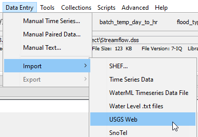
Open the USGS Download editor by selecting Data Entry | Import | USGS Web.
Enter the USGS Station ID for the specific station of interest within the USGS Station ID's column, 11132500.
Enter the River Name within the Basin Name (A Part) column, Salsipuedes Creek.
Enter the Gage Name within the Location (B Part) column, Lompoc.
Enter USGS within the Other Qualifier (F Part) column.
Click the checkbox within the Import Data column. The selections should appear as in the figure below.
Import Instantaneous Data:
1. Change the Data Type to Instantaneous (15-min, hourly) using the drop-down menu.
2. Enter a start and end date/time that encompasses the flood event in question, 14Feb2017:0000 to 25Feb2017:0000.
3. Set the Select Time Zone Option to UTC.
4. Click the Import to DSS button to import instantaneous data.
Import Annual Maximum Series:
1. Once the data has been imported, change the Data Type to Annual Peak Data.
2. Click the Import to DSS button to import the annual maximum series
3. Close the USGS Download editor
(Optional) Convert Irregular Data to Regular Data:
1. To be used if the E Part uses a tilde character, as shown below.
2. Select the time series of interest.
3. Click Tools | Math Functions.
4. Select the Time Functions tab.
5. Select the Irregular to Regular operator.
6. Ensure the Interpolate radio button is selected.
7. Ensure the Time Interval is set to an appropriate value (i.e. a time interval similar to the value after the tilde character in the original data set is a good first guess).
8. Click Compute.
9. Click the Save button
10. Delete the time series that has a tilde character within the E Part.
Delete unnecessary data:
1. Do not delete any records containing "FLOW" in the C Part.
2. Once all unnecessary time series have been deleted, click Tools | Squeeze.
View the data:
1. Select the annual maximum series and instantaneous flow data.
2. Click the Plot button .
3. The data should resemble the figure below, note that the default line styles were changed within this figure.
  
  When using HEC-DSSVue, Annual Peak Data is imported in local time, as specified in USGS peak flow files. While this annual peak event was not recorded with an associated time (simply recorded at the end of the day 17 February 2017, 24:00), it is important to be aware of time zone discrepancies. The time zone conversion for this watershed in February is: Pacific Standard Time (PST) + 8 hr = Coordinated Universal Time (UTC).

Delineate Modeling Elements Using HEC-HMS

Ensure you are using HEC-HMS v4.7 (or more recent), which can be downloaded here: https://www.hec.usace.army.mil/software/hec-hms/downloads.aspx
Create a new HEC-HMS project:
1. Name the project after the watershed in question, Salsipuedes_Creek.
2. Make sure the Default Unit System is set to U.S. Customary.
3. Move the GIS folder into the project's maps directory.
Create a new Basin Model:
1. Click Components | Basin Model Manager | New.
2. Name the Basin Model Feb_2017 according to the event in question.
Create a new Terrain Data component:
1. Click Components | Terrain Data Manager | New.
2. Name it NED_10m.
3. Select the NED_10m_alb_clip_ft.tif dataset, in the GIS folder.
4. Set the Vertical Units to Feet
5. Click Finish.
Select the Terrain Data within the Basin Model's Component Editor:
1. Click the Save button.
2. Click Skip to use the coordinate system from the terrain data.
3. The terrain data should now appear within the Map.
4. Right click on the Map window to use the Map Layers... editor and add the NHDFlowLine, Stream_Gage, and WBD_HUC12 shapefiles to the basin model
5. Edit the shapefile draw properties until you are satisfied with the GIS display.
Fill sinks using the GIS | Preprocess Sinks tool.
Compute flow directions and flow accumulations using the GIS | Preprocess Drainage tool.
Compute stream locations using the GIS | Identify Streams tool.
1. Use a stream threshold that is slightly less than the reported drainage area of the gage of interest, 45 sq. mi. for Salsipuedes Creek (reported drainage area = 47 sq. mi.). This will minimize the amount of subbasin splitting/merging that will need to be performed later.
Add a breakpoint at the stream gage location that was added as a map layer using the Breakpoint tool .
1. Zoom into the stream gage location and make sure you add the break point on top of a cell within the identified streams layer (you might need to modify the draw properties and turn off some Map Layers to better see the identified streams grid cells). The stream gage may not fall directly on an identified streams cell, however, create the breakpoint as close as possible to the gage location.
2. Name the breakpoint Outlet.
Delineate Elements using the GIS | Delineate Elements tool:
1. Use a Subbasin Prefix of S_
2. Use a Reach Prefix of R_
3. Set Insert Junctions to Yes
4. Use a Junction Prefix of J_
5. Set Convert Break Points to Yes. This will create a sink at the Outlet breakpoint.
Click View | Map Layers to open the Map Layers Dialog.
1. Turn off all layers except Icons, Subbasins, Discretization, Terrain, and the three shapefiles
Rename the subbasin element.
1. An appropriate subbasin names is "SalsipuedesCk_S10"
Rename the sink element to Outlet.
Ensure the subbasin drainage area is approximately equivalent to the reported drainage area.
Set subbasin modeling processes:
1. Structured discretization method
2. Deficit and Constant loss method
3. Clark Unit Hydrograph transform method
4. Linear Reservoir baseflow method
Compute Grid Cells for the subbasin element(s):
1. On the Discretization tab, ensure the Projection is set to SHG and the Cell Size is set to 2000.
2. Click GIS | Compute | Grid Cells.
3. The grid cells (i.e. discretization) should be shown in the Map Panel.

Parameterize the Subbasin Element

Run the Subbasin Characteristics tool from Parameters | Characteristics | Subbasin to compute the longest flowpath, centroidal flowpath, and flowpath slope characteristics.
Use the parameter calculator (accessed from Parameters | Transform menu) to estimate the Clark time of concentration using the following equation:

$\begin{array}{l}\displaystyle T_c = 2.2 * (\frac{L*L_C}{\sqrt{Slope_{10-85}}})^{0.3}\end{array}$

where $\begin{array}{l}T_c\end{array}$ = time of concentration (hrs); $\begin{array}{l}L =\end{array}$ longest flow path (mi); $\begin{array}{l}L_c\end{array}$ = Centroidal flow path (mi); $\begin{array}{l}Slope_{10-85}\end{array}$ = average slope of the flow path represented by 10 to 85 percent of the longest flow path (ft/mi).
You can find out more about estimating the Clark time of concentration and storage coefficient parameters here.
Round the time of concentration to the nearest tenth.

Populate the remaining initial subbasin parameter values (soil and landuse data could be used to improve initial estimates)

The table below contains initial parameter estimates.
Enter the initial loss parameters for the subbasin.
Enter the initial storage coefficient for the subbasin.
1. Set the Method to Standard.
2. Set the Time-Area Method to Default.

Enter the initial Linear Reservoir baseflow parameters for the subbasin

Set the Layers (number of reservoirs) to 2.

Set the Initial Type to Discharge Per Area.

Loss Parameters	Initial Parameter Values
Initial Deficit (in)	0
Maximum Deficit (in)	8
Constant Rate (in/hr)	0.1
Percent Impervious Area	0
Transform Parameters
Time of Concentration (hrs)	Estimate from Characteristics / Regression Eqn.
Storage Coefficient (hrs)	R / (R + TC) = 0.5
Baseflow Parameters
GW1 Initial (cfs/sq mi)	0
GW1 Fraction	0.5
GW1 Coefficient (hrs)	Three times larger than R
GW1 Steps	1
GW2 Initial (cfs/sq mi)	0
GW2 Fraction	0.5
GW2 Coefficient (hrs)	Ten times larger than R
GW2 Steps	1

Add Streamflow and Precipitation Data to the Project

If needed, within the newly created HEC-HMS project directory, add a new subdirectory called "Data" (depending on HEC-HMS version, the "data" directory may already exist).
1. This subdirectory should be placed within the project directory.
2. Copy the MRMS_Precipitation.dss file to this new directory.
3. Copy the Streamflow.dss file to this new directory.
Within HEC-HMS, create a new Time Series Discharge Gage.
1. Click Components | Time-Series Data Manager.
2. Select Discharge Gage.
3. Click the New... button.
4. Name the new gage after the location of interest, SalsipuedesCk_nr_Lompoc.
5. Select the newly created discharge time series gage in the Watershed Explorer.
6. Set the Data Source to Single Record HEC-DSS.
7. Select the DSS Filename and DSS Pathname that correspond to the 15-minute observed streamflow data, the time series that uses an E Part of 15Minute.
Set observed data within the basin model.
1. Select the Sink element that represents the gage location (Outlet).
2. In the Component Editor, on the Options tab:
  1. Enter the annual peak discharge that was downloaded from the USGS within the Ref Flow =field.
  2. Enter an appropriate text string within the Ref Label field.
  3. Select the newly created time series discharge gage within the Observed Flow drop down menu.
  4. The Options tab should resemble the figure below.
Create a new precipitation gridset.
1. Click Components | Grid Data Manager.
2. Select Precipitation Gridsets.
3. Click the New... button.
4. Name the new grid after the source of data, MRMS.
5. Select the newly created Precipitation Grid in the Watershed Explorer.
6. Set the Data Source to Single Record HEC-DSS.
7. Select the DSS Filename and DSS Pathname that corresponds to the MRMS precipitation data

Calibrate the Model

Create a new Meteorologic Model
1. Click Components | Meteorologic Model Manager.
2. Click the New... button.
3. Name the new Meteorologic Model after the source of data, MRMS.
Populate the Meteorologic Model components.
1. Select the newly created Meteorologic Model.
2. Set the Unit System to U.S. Customary.
3. Set the Shortwave, Longwave, Temperature, Windspeed, Pressure, Dew Point, and Evapotranspiration methods to --None--.
4. Set the Precipitation method to Gridded Precipitation.
5. Set Replace Missing to Set To Default.
6. The Meteorologic Model Component Editor should resemble the figure below.
7. Navigate to the Basins tab (if present - version 4.9 and newer do not require linking Met Model to the Basin Model unless the meteorology needs subbasin-level parameterizations).
8. Select the corresponding Basin Model in the Include Subbasins column.
9. Select the Gridded Precipitation node.
10. Select MRMS from the Grid Name drop down menu.
11. Make sure the Time Shift Method is set to --None--.
Create a new Control Specifications.
1. Click Components | Control Specifications Manager.
2. Click the New... button.
3. Name the new Control Specifications after the event in question, Feb_2017.
4. Click the Finish button.
5. Select the newly created Control Specifications in the Watershed Explorer.
6. Set the Start Date, Start Time, End Date, and End Time for the event, 16Feb2017:1200 to 24Feb2017:0000.
7. Set the Time Interval to 15 Minutes.
Create a new Simulation Run.
1. Click Compute | Create Compute | Simulation Run....
2. Name the simulation run after the event, e.g. Feb_2017.
3. Select the newly created Basin Model.
4. Select the newly created Meteorologic Model
5. Select the newly created Control Specifications.
Compute the simulation and compare the computed results against the observed data.
Modify Baseflow parameters (GW 2 Initial) to match the observed discharge at the beginning of the simulation.

Iteratively modify Loss, Transform, and Baseflow parameters to achieve a Satisfactory, Good, or Very Good (preferred) NSE, RSR (RMSE Std Dev), and Percent Bias rating. Keep track of the parameter modifications.

Start by modifying parameters that control the simulated runoff at the start of the simulation (e.g., GW 1 Initial, GW 2 Initial, and Initial Deficit).
Modify Loss parameters (Initial Deficit and Constant Rate) and Baseflow parameters (GW 1 Fraction and GW 2 Fraction) to approximately match the initiation of runoff and observed discharge volume.

Modify Transform parameters (Time of Concentration and Storage Coefficient) to approximately match the peak discharge, time of peak discharge, and overall shape of the observed discharge hydrograph.

Performance Rating	NSE	RSR	PBIAS
Very Good	0.65<𝑁𝑆𝐸≤1.00	0.00<𝑅𝑆𝑅≤0.60	𝑃𝐵𝐼𝐴𝑆< ±15
Good	0.55<𝑁𝑆𝐸≤0.65	0.60<𝑅𝑆𝑅≤0.70	±15≤𝑃𝐵𝐼𝐴𝑆<±20
Satisfactory	0.40<𝑁𝑆𝐸≤0.55	0.70<𝑅𝑆𝑅≤0.80	±20≤𝑃𝐵𝐼𝐴𝑆<±30
Unsatisfactory	𝑁𝑆𝐸≤0.40	𝑅𝑆𝑅>0.80	𝑃𝐵𝐼𝐴𝑆≥±30

The final results should resemble the figure below.

Document Final Model Parameters

Enter final model parameters in the table below.

Loss Parameters	Initial Parameter Values	Final Parameter Values
Initial Deficit (in)	0
Maximum Deficit (in)	8
Constant Rate (in/hr)	0.1
Percent Impervious Area	0
Transform Parameters
Time of Concentration (hrs)	Estimate from Characteristics / Regression Eqn.
Storage Coefficient (hrs)	R / (R + TC) = 0.5
Baseflow Parameters
GW1 Initial (cfs/sq mi)	0
GW2 Initial (cfs/sq mi)	0
GW1 Fraction	0.5
GW1 Coefficient (hrs)	Three times larger than R
GW1 Steps	1
GW2 Fraction	0.5
GW2 Steps	1
GW2 Coefficient (hrs)	Ten times larger than R

Answer the following questions and share your thoughts with others:
1. Describe the process you followed to calibrate the model.
2. What was the most challenging part of model development and calibration?
3. How much confidence do you have in the initial parameter estimates?
4. Which parameters had the greatest impact on the computed results? Which parameters had the least impact on the computed results?

Submit your results spreadsheet here in the format LastName_FirstName: November 2024 Basic HMS - Files - HEC Drive