Download PDF
Download page W2 - Applying the Clark/ModClark Unit Hydrograph Method.
W2 - Applying the Clark/ModClark Unit Hydrograph Method
Overview
In this workshop you will apply the HEC-HMS ModClark unit hydrograph method to a modeling application. Initial parameter estimates will be estimated using GIS information and the model will be calibrated through trial and error. Uncertainty in hydrologic model outputs due to the estimated unit hydrograph parameters will also be quantified. HEC-HMS version 4.9 was used to created this workshop. You will need to use HEC-HMS version 4.9, or newer, to open the project files.
Download the initial project files here - start_Clark_UH_Workshop.zip
Background
The Clark unit hydrograph method utilizes the concept of an instantaneous unit hydrograph to route excess precipitation to the subbasin outlet. An instantaneous unit hydrograph is derived by instantaneously applying a unit depth (e.g. one inch) of excess precipitation over a watershed (Clark, 1945). The resultant unit hydrograph is entirely theoretical (i.e. real precipitation cannot be applied instantaneously to a watershed) but it has the distinct advantage of characterizing the watershed’s response to rainfall without reference to the duration of excess precipitation (Chow, Maidment, & Mays, 1988). This method explicitly represents two critical processes in the transformation of excess precipitation to runoff: 1) the translation (or movement) of excess precipitation from its origin throughout the watershed to the outlet and 2) the attenuation (or reduction) of the magnitude of the discharge as the excess precipitation is temporarily stored throughout the watershed (U.S. Army Corps of Engineers, 2021). Conceptually, water is translated from remote points to the watershed outlet with delay but without attenuation. Attenuation is then incorporated, conceptually speaking, at the watershed outlet. Three parameters are utilized within this method:
- Time of concentration (Tc), which is equivalent to the time it takes for excess precipitation to travel from the hydraulically-most remote point of the watershed to the outlet,
- Watershed storage coefficient (R), which is equivalent to attenuation due to storage effects throughout the watershed (Kull & Feldman, 1998), and
- Time-Area histogram, which represents the watershed area that contributes to flow at the outlet as a function of time.
The Modified Clark (ModClark) method explicitly accounts for variations in travel time to the watershed outlet using a gridded representation of the watershed to route excess precipitation to the subbasin outlet (Kull & Feldman, 1998). While the method integrates spatial variability in travel time, the underlying flow velocity field is time invariant. The travel time index for each grid cell, T_{t, \text { cell }}, is set relative to the time of concentration for the watershed, T_{c, \text { watershed }}, using a distance index:
| T_{t, \text { cell }}=T_{c, \text { watershed }} \frac{D_{c e l l}}{D_{\max }} |
where D_{c e l l} is the travel distance from a grid cell to the watershed outlet and D_{\max } is the travel distance for the grid cell that is most distant from the watershed outlet. As long as the area for each grid cell is also specified, the volume of inflow can be computed as the product of area and excess precipitation. This, in essence, creates a watershed-specific time-area histogram instead of using a smooth function fitted to a typical time-area relationship. Inflows are then routed through a linear reservoir yielding an outflow hydrograph for each grid cell. The current implementation within HEC-HMS assumes the watershed storage coefficient, R, is uniform throughout each grid cell for a watershed (Hydrologic Engineering Center, 2018). The individual outflow hydrographs from each grid cell are then summed to determine the total direct runoff hydrograph.
Regression equations that can be used to predict Clark and ModClark unit hydrograph parameters were developed for the state of California as part of Task 5 within the Memorandum of Agreement between HEC and DSOD. These equations relate physically measurable watershed characteristics (e.g. longest flow path) to time of concentration and storage coefficient. Separate regression equations were developed for time of concentration and watershed storage coefficient.
Extract Basin Characteristics and Estimate Time of Concentration and Storage Coefficient
- Open the Clark_UH_Workshop project and then open the Dec_1996_Jan_1997 Basin Model.
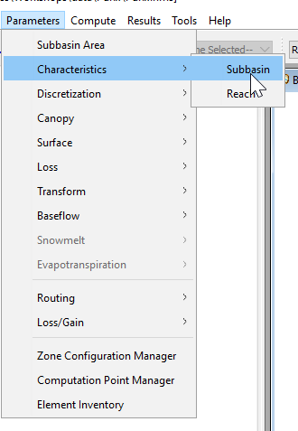
- Compute basin characteristics for the selected basin model by selecting Parameters | Characteristics | Subbasin, as shown within the following figure.
HEC-HMS will populate characteristics for each subbasin element within the basin model, as shown within the following figure.

- Using the equations and basin characteristics, calculate Tc and R for the subbasin of interest.
Question 1: What are the estimated Tc and R values for this subbasin?
Tc = 3.2 hrs and R = 2.9 hrs
Enter Parameter Values and Compute a Simulation
Now that you have estimated Tc and R values for the MF_American_Rv_S30 subbasin, you need to apply them within the HEC-HMS project.
- Select the MF_American_Rv_S30 subbasin element.
- Select the Transform tab to open the ModClark Component Editor.
- Enter the Tc and R values that were estimated in the previous section. The ModClark Component Editor should resemble the following figure.

- Select the Discretization tab to open the Structured Discretization Component Editor.
- Ensure that the SHG Projection and 2000 meter Cell Size is selected. The Structured Discretization Component Editor should resemble the following figure.
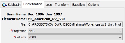
- Click GIS | Compute | Grid Cells. You should notice that a set of grid cells overlying the MF_American_Rv_S30 subbasin element are now displayed. If you do not see these grid cells, click View | Map Layers and toggle on the Discretization layer.
- Select the Dec_1996_Jan_1997 simulation run from the Compute toolbar.
- Press the Compute All Elements button to run the simulation.
- Once the compute is complete, investigate the initial results
- Try viewing the result graph and summary table for the MF_American_Rv_S30 subbasin element.
- Also, try navigating to the Results tab, expanding the Simulation Runs node, clicking on the Dec_1996_Jan_1997 node, and selecting the MF_American_Rv_S30 node.
- Select the Outflow, Direct Runoff, and Baseflow time series, as shown within the following figure.
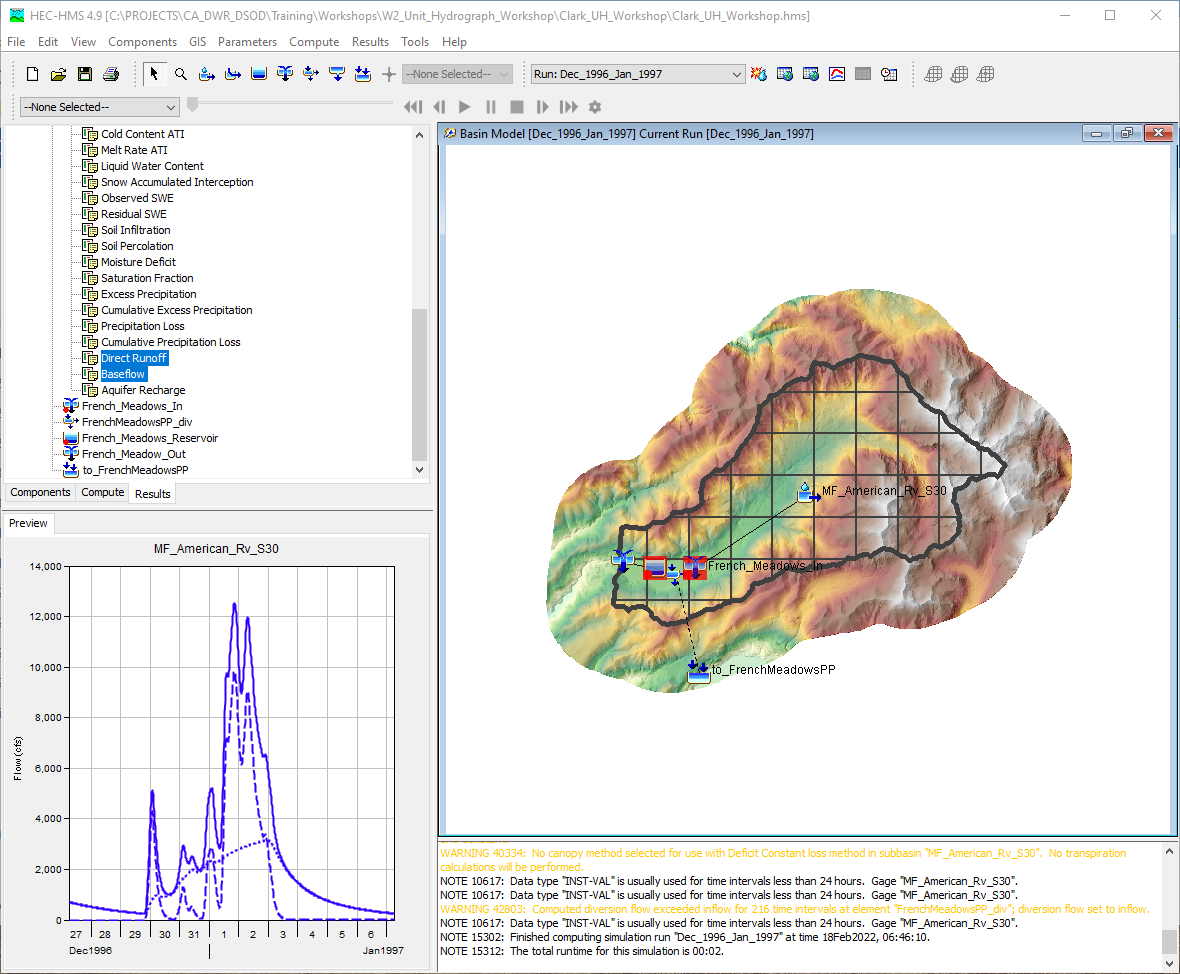
- These plots can also be opened in a stand-alone frame by clicking the result graph button.
Question 2: Which of these three time series depend upon the Tc and R values that were previously entered?
The Direct Runoff and Outflow time series depend upon the input Tc and R values. Since the Linear Reservoir baseflow method was selected, the Baseflow time series does not depend upon the Tc and R values.
Question 3. Is the Direct Runoff time series a "unit hydrograph"? Why or why not? If not, how would you go about generating a unit hydrograph in HEC-HMS?
No. A unit hydrograph is defined as "the basin outflow resulting from one unit of direct runoff generated uniformly over the drainage area at a uniform rainfall rate during a specified period of rainfall duration" (Sherman, 1932). The Direct Runoff time series contains more than one inch of runoff. Also, this time series is the composition of multiple, temporally varying, pulses of excess precipitation each of which were routed using a unit hydrograph for the subbasin.
You can generate a unit hydrograph by turning off any losses (or setting losses to zero), turning off or removing the baseflow component, inputting one inch of precipitation in the meteorological model over the entire basin, and simulating the model.
Calibrate the Model
Calibrating a model to afford better agreement between computed and observed runoff oftentimes requires simultaneous changes to more than just one process (e.g. calibrate loss, transform, and baseflow at the same time). However, within this workshop, only the ModClark unit hydrograph transform parameters will be modified.
- In general, calibration of transform parameters should proceed by first attempting to approximately match the rising limb of the observed data, then continue modifying parameters to approximately match the receding limb of the observed data, and finally attempting to simultaneously best match the rising limb, peak pool elevation/discharge, and receding limb of the observed data.
- The following outputs should be used to ascertain the effectiveness and appropriateness of each change:
- View the result graph and summary table for the MF_American_Rv_S30 subbasin element.
- View a graph of cumulative flow for the MF_American_Rv_S30 subbasin element.
On the Results tab | Simulation Runs node | Dec_1996_Jan_1997 node | MF_American_Rv_S30 node, select the Outflow, Cumulative Outflow, Observed Flow, and Cumulative Observed Flow time series, as shown in the following figure.
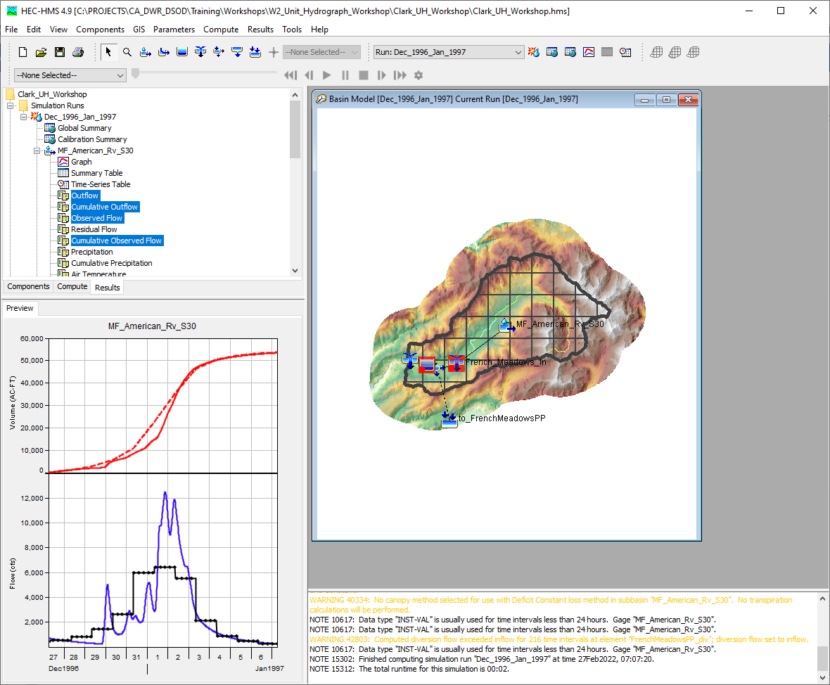
Click the result graph button to open this plot within a stand alone frame.
- View the result graph and summary table for the French_Meadows_Reservoir reservoir element.
- Try the following parameter combinations:
- Increasing Tc by a factor of 5 and leaving R unchanged (Tc = 16 hrs, R = 2.9 hrs)
- Halving Tc and leaving R unchanged (Tc = 1.6 hrs, R = 2.9 hrs)
- Leaving Tc unchanged and increasing R by a factor of 5 (Tc = 3.2 hrs, R = 14.5 hrs)
- Leaving Tc unchanged and halving R (Tc = 3.2 hrs, R = 1.5 hrs)
- Compare the results at the MF_American_Rv_S30 and French_Meadows_Reservoir elements after each change.
Question 4. What happens (in terms of hydrograph peak, shape, and timing) when you change Tc? How did the computed results compare to the observed data for each change? Which value provides the best agreement with the observed data?
The time of concentration is the time it takes for water to travel from the most remote point in the watershed to the watershed outlet (pourpoint). By reducing Tc, the hydrograph arrives at the outlet sooner. Conversely, increasing Tc results in the computed hydrograph shifting to the right meaning water arrives at the watershed outlet later.
When using a Tc of 16 hrs, the computed hydrograph is much smoother, the computed results are translated later in time, and the peak discharge/pool elevation is lower than when using the initial estimates. When using a Tc of 1.6 hrs, the computed results are essentially the same as the initial results.
Due to the use of daily average data, it's difficult to ascertain the optimal Tc. Also, simultaneously matching peak reservoir pool elevation, runoff volume, and hydrograph shape can be difficult. To better match the observed data, modifications to snowmelt, loss, unit hydrograph, and/or baseflow parameters may be necessary.
Question 5. What happens (in terms of hydrograph peak, shape, and timing) when you change R? How did the computed results compare to the observed data for each change? Which value provides the best agreement with the observed data?
The storage coefficient is a representation of temporary water storage. By reducing R, the hydrograph shape "narrows" (the rising limb and recession limb have a steeper slope) causing the peak value to increase while also shifting the time to peak earlier in time. By increasing R, the hydrograph shape "flattens" or attenuates which reduces the hydrograph peak and extends the recession limb of the hydrograph later in time.
When using an R of 14.5 hrs, the computed hydrograph is much smoother, the computed results are translated later in time, and the peak discharge/pool elevation is lower than when using the initial estimates (even more so than when using a Tc of 16 hrs). When using an R of 1.5 hrs, the computed results are essentially the same as the initial results.
Due to the use of daily average data, it's difficult to ascertain the optimal R. Also, simultaneously matching peak reservoir pool elevation, runoff volume, and hydrograph shape can be difficult. To better match the observed data, modifications to snowmelt, loss, unit hydrograph, and/or baseflow parameters may be necessary.
Estimate Uncertainty in the Model Outputs due to Transform Parameters
The regression equations presented within the previous sections represent the most likely Tc or R value for a given location. However, the regression equations contain uncertainty which cannot be completely eliminated. To quantify the amount of uncertainty present when estimating a Tc or R for a specific location, prediction intervals can be estimated using the following equation:
| y^{*} \pm t_{\alpha / 2, n-2)} \sqrt{M S E+\left[S E\left(y^{*}\right)\right]^{2}} |
where y^{*} = predicted value (Tc or R), t_{\alpha / 2, n-2)} = t distribution critical value, n = number of observations, and M S E+\left[S E\left(y^{*}\right)\right]^{2} = the standard error of the prediction. Prediction intervals should be used when estimating the uncertainty around a yet-to-be-observed data point since they incorporate both the model parameter uncertainty (e.g. error around the population mean at the input value) in addition to the residual uncertainty.
When using weighted multiple linear regression, as is the case within this study, the estimation of the standard error of the prediction is complex. As such, statistical software (e.g. R Statistical Language) was used to estimate prediction intervals for the MF_American_Rv_S30 subbasin. These values are shown below.
| Value | Tc (hr) | R (hr) |
|---|---|---|
| Predicted | 3.2 | 2.9 |
| Upper Prediction Limit | 9.1 | 24.9 |
| Lower Prediction Limit | -2.6 | 0.3 |
Prediction intervals can be used to estimate the amount of uncertainty in hydrologic model outputs (e.g. runoff volume, peak discharge, peak reservoir elevation, etc) that is due to use of Clark unit hydrograph parameters predicted using the regression equations. Due to the use of linear regression, uncertainty about any predicted Tc or R value is assumed to be normally distributed.
Question 6. Parameterize a normal distribution for Tc (i.e. estimate a mean and standard deviation).
The mean is equivalent to the predicted value (3.2 hrs).
The Empirical Rule can be used to estimate the standard deviation. Specifically, this rule states that two standard deviations encompass 95% of the data and 68% covers one standard deviation. The 95% prediction interval encompasses 11.7 hrs (i.e. 9.1 minus -2.6 hrs). Given this information, you can estimate one standard deviation using a simple ratio (i.e. 11.7 hrs * 68 / 95 = 8.4 hrs).
Question 7. Parameterize a normal distribution for R (i.e. estimate a mean and standard deviation).
The mean is equivalent to the predicted value (2.9 hrs).
The Empirical Rule can be used to estimate the standard deviation (i.e. 24.6 hrs * 68 / 95 = 17.6 hrs).
HEC-HMS contains the ability to sample from one or more probability distributions representing uncertain parameters. However, within this example, instead of inputting the parameterized distributions you just developed within HEC-HMS, a sequence of random Tc and R values were developed external to HEC-HMS. Then, these random Tc and R values were input to HEC-HMS as Parameter Value Samples, which can also be used within an Uncertainty Analysis, as shown in the following figure.
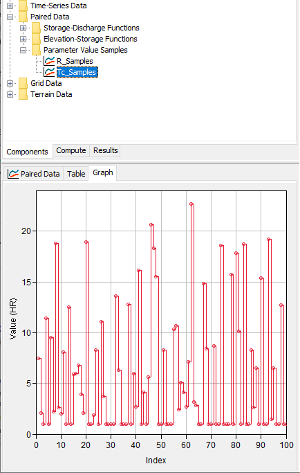
Download the file that was used to generate the random Tc and R samples here - sample_generation.xlsx
- Begin assessing parameter uncertainty by creating a new Uncertainty Analysis.
- Click Compute | Create Compute | Uncertainty Analysis.
- Name the new simulation run "Clark_Uncertainty".
- Select the Dec_1996_Jan_1997 basin model.
- Select the GriddedData_1997 meteorologic model.
- Click Finish to create the Uncertainty Analysis.
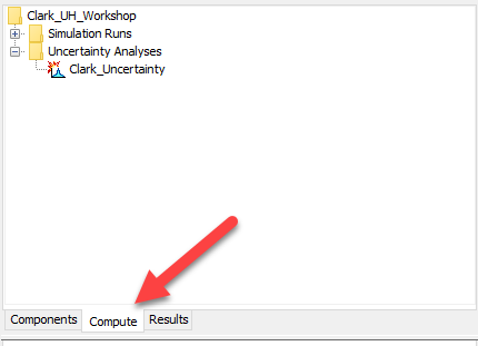
- Switch to the Compute tab, as shown within the following figure.
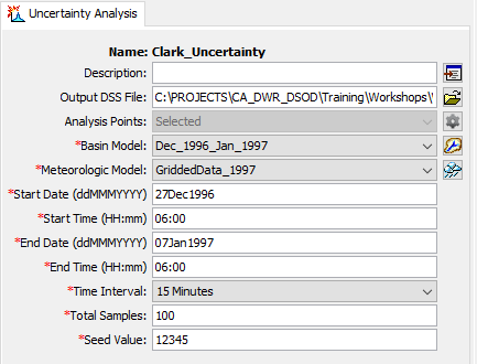
- Select the "Clark_Uncertainty" node and enter a Start Date, Start Time, End Date, End Time, Time Interval,Total Samples, and Seed Value as shown within the following figure.
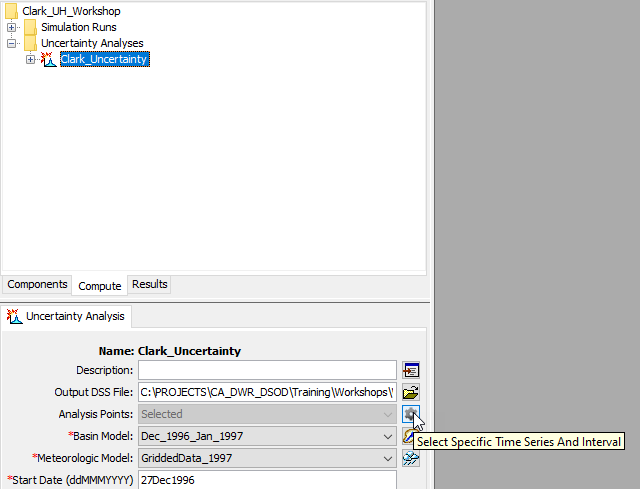
- Click on the Analysis Points selection button, as shown within the following figure.
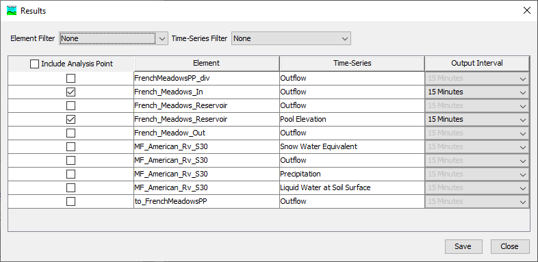
- Select the French_Meadows_In | Outflow and French_Meadows_Reservoir | Pool Elevation time series, as shown within the following figure. Click Save and Close to close the dialog.
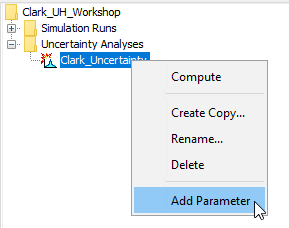
- Right-click on the "Clark_Uncertainty" node and click Add Parameter, as shown within the following figure.
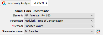
Click on the "Parameter 1" node.
Select the MF_American_Rv_S30 element, ModClark - Time of Concentration parameter, Specified Values method, and Tc_Samples parameter value, as shown within the following figure.
- Right-click on the "Clark_Uncertainty" node and click Add Parameter.
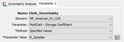
- Click on the "Parameter 2" node.
- Select the MF_American_Rv_S30 element, ModClark - Storage Coefficient parameter, Specified Values method, and R_Samples parameter value, as shown within the following figure.
- Select the MF_American_Rv_S30 element, ModClark - Storage Coefficient parameter, Specified Values method, and R_Samples parameter value, as shown within the following figure.
- Select the Clark_Uncertainty analysis from the Compute toolbar,
 .
. Press the Compute All Elements button to run the analysis.
The Uncertainty Analysis should take approximately two minutes to complete all 100 iterations.
- Switch to the Results tab, expand the Uncertainty Analyses node, click on the Clark_Unceratinty node, and investigate the results.
- The Parameter 1 node contains the sampled values for Tc.
- The Parameter 2 node contains the sampled values for R.
- The French_Meadows_In node contains the output time series that were saved for the French_Meadows_In junction element.
- The French_Meadows_Reservoir node contains the output time series that were saved for the French_Meadows_Reservoir reservoir element.
- Investigate the results and answer the following questions:
Question 8. How much variability within the peak inflow to French Meadows Reservoir is due to the unit hydrograph parameters?
The inflow to French Meadows Reservoir is contained within the "French_Meadows_In" results graph, which is shown within the following figure. Within this figure, mean (solid dark blue line), mean +/- 1 standard deviation (dashed dark blue lines), and minimum/maximum (dashed light blue line) outflow hydrographs are displayed.
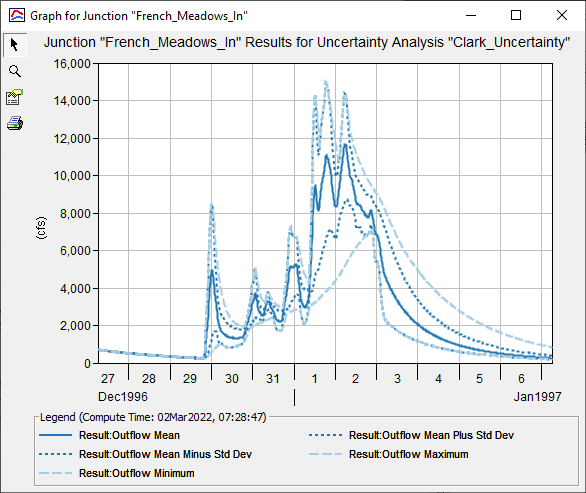
The largest peak discharge that was realized during this analysis is approximately 15000 cfs while the minimum peak discharge is approximately 7000 cfs. The difference between these two values is approximately 8000 cfs.
Question 9. How much variability within the peak pool elevation at French Meadows Reservoir is due to the unit hydrograph parameters?
The pool elevation at French Meadows Reservoir is contained within the "French_Meadows_Reservoir" results graph, which is shown within the following figure. Within this figure, mean (solid dark blue line), mean +/- 1 standard deviation (dashed dark blue lines), and minimum/maximum (dashed light blue line) outflow hydrographs are displayed.
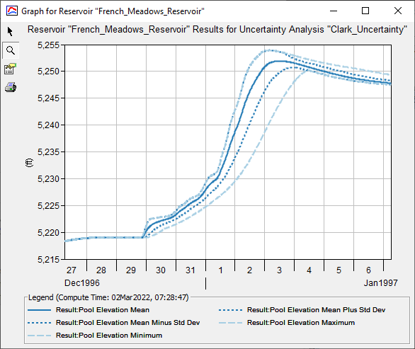
The largest peak pool elevation that was realized during this analysis is approximately 5254 ft NGVD29 while the minimum peak pool elevation is approximately 5250.25 ft NGVD29. The difference between these two values is approximately 3.75 ft.
Question 10. Which parameters were sampled/varied during this Uncertainty Analysis? Which parameters WERE NOT sampled?
Only Tc and R were sampled during this analysis. No other parameters were sampled. For instance, precipitation depth, daily maximum temperature, infiltration, and baseflow parameters were not varied. Within a real study, these parameters should also be randomly sampled to investigate their contribution to uncertainty in hydrologic outputs of interest.
To sample from uncertain meteorologic boundary conditions, applications like HEC-WAT can be used in concert with HEC-HMS.
For more information pertaining to the Uncertainty analysis within HEC-HMS, users are directed to the Assessing Model Uncertainty section within the HEC-HMS user’s manual: https://www.hec.usace.army.mil/confluence/hmsdocs/hmsum/latest/assessing-model-uncertainty.
Download the final project files here - finish_Clark_UH_Workshop.zip
Additional Task - Compute Tc and R using the Expression Calculator
- Open the ModClark unit hydrograph transform global editor by selecting Parameters | Transform | ModClark.
- Within the global editor, click the Calculator button located near the bottom of the frame to open the Expression Calculator.
- Within the Expression Calculator, ensure that Time of Concentration is the selected field.
Within the expression entry field, enter the regression equation for Tc
- Click Calculate.
- After calculating, the global editor will fill with the computed Tc value.
Repeat steps 3 - 5 to estimate R.
Additional Task - Estimate Prediction Intervals using the R Statistical Language
Prediction intervals can be calculated using the following equation:
| y^{*} \pm t_{\alpha / 2, n-2)} \sqrt{M S E+\left[S E\left(y^{*}\right)\right]^{2}} |
where y^{*} = predicted value (Tc or R), t_{\alpha / 2, n-2)} = t distribution critical value, n = number of observations, and \sqrt{M S E+\left[S E\left(y^{*}\right)\right]^{2}} = the standard error of the prediction. When using weighted multiple linear regression, the estimation of the standard error of the prediction is complex. As such, statistical software (e.g. R Statistical Language) should be used to estimate prediction intervals. An example of this analysis is shown in the following code block.
rm(list = ls())

library(readr)
library(tidyverse)
library(GGally)

setwd(<insert the location of the "Master_Parameter_Summary.csv" file here>)

master_parameters <- read_csv("Master_Parameter_Summary.csv")
regionData <- master_parameters %>%
  filter(RegionNumber == 2 | RegionNumber == 3 | RegionNumber == 4 |
           RegionNumber == 6 | RegionNumber == 7)

validation_data <- data.frame(LSqrtDAS=875.9354)

Tc_vs_LSqrtDAS <- lm(Tc ~ LSqrtDAS, data = regionData, weights = Weight)

summary(Tc_vs_LSqrtDAS)

predict(Tc_vs_LSqrtDAS, validation_data, interval = "prediction", level = 0.95)