W4 - Applying the Muskingum-Cunge Routing Method

Overview

In this workshop you will apply the HEC-HMS Muskingum-Cunge channel routing method to a modeling application. Initial parameter estimates will be estimated using GIS and observed information and the model will be calibrated through trial and error. HEC-HMS version 4.9 was used to create this workshop. You will need to use HEC-HMS version 4.9, or newer, to open the project files.

Download the initial project files here - start_Muskingum_Cunge_Workshop.zip

Background

The Muskingum-Cunge routing method builds upon concepts within the Muskingum method. This method uses a combination of the continuity equation and a simplified form of the momentum equation. Within the previously mentioned Muskingum method, the X parameter is a dimensionless coefficient that lacks a strong physical meaning. Cunge (1969) evaluated the numerical diffusion that is produced through the use of the Muskingum routing equation and set this equal to the physical diffusion represented by the convective diffusion equation (Miller & Cunge, 1975). The Muskingum-Cunge method is sometimes referred to as a “variable coefficient” method since the routing parameters are recalculated every time step based upon channel properties and the flow depth.

Estimate Initial Parameter Values

Reach Length

The reach length should be set as the total length of the reach element. This parameter is typically estimated using GIS information and field survey data, when available. The total length of the reach in question is approximately 8.3 miles and is shown in the following figure.

Stream Miles

Friction Slope

The friction slope should be set as the average friction slope for the entire reach. If the friction slope varies significantly throughout the stream represented by the reach, it may be necessary to use multiple reaches with different slopes. If no information is available to estimate the friction slope, the bed slope can be used as an approximation. This parameter is typically estimated using GIS information and field survey data, when available. In this workshop, invert elevations were extracted along the reach of interest and are shown in the following figure. The profile data for this information is detailed in the following table.

MF_American_Rv_R20 Profile

Profile Data for MF_American_Rv_R20

Station (mi)	Elevation (ft)
0	3345
0.5	3486
1	3586
1.5	3718
2	3797
2.5	3889
3	3973
3.5	4053
4	4128
4.5	4204
5	4309
5.5	4436
6	4535
6.5	4655
7	4793
7.5	4904
8	5014
8.3	5100

Question 1: Estimate a single, representative slope (in ft/ft) for the reach in question.

Bed slopes throughout the reach vary between a minimum of 0.028 ft/ft and a maximum of 0.053 ft/ft, as shown in the following plot. These changes are relatively minor. Thus, a single, representative slope for this reach appears to be an appropriate assumption.

To calculate a single slope, the change in elevation can be divided by the length of the reach:

$\begin{array}{l}Slope = \frac{Rise}{Run}\end{array}$

$\begin{array}{l}Slope = \frac{5100 ft - 3345 ft}{43890 ft}\end{array}$

$\begin{array}{l}Slope = 0.04 \frac{ft}{ft}\end{array}$

Manning's n Roughness Coefficient

The Manning's n roughness coefficient(s) should be set as the average value for the whole reach. Depending upon the cross section shape that is chosen, zero , one, or three Manning's n roughness coefficients are required. This parameter is typically estimated using “reference” streams with established roughness coefficients or through model calibration.

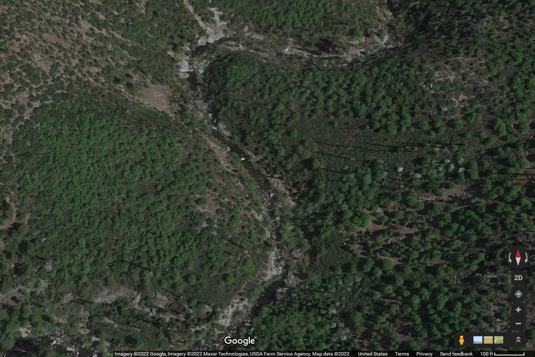
The reach of interest is winding, very steep, and has little to no overbank storage. The channel is comprised of granitic stones and some boulders, as shown in the following image.

Manning's roughness values for reference streams are published in many sources. The following table of typical Manning's roughness values was published in Chow (1959).

Typical Manning's Roughness Coefficients (from Chow, 1959)

Question 2. Estimate Manning's roughness coefficients for both the main channel and overbank areas.

Manning's roughness coefficients of 0.035 and 0.05 can be reasonably assumed for the main channel and overbank areas, respectively.

Keep in mind that these are initial estimates and should be calibrated using observed data.

Space-Time Interval

The choice of space and time steps (Δx and Δt, respectively) are critical to ensure accuracy and stability. Three options for specifying a space-time method are provided within HEC-HMS:

Auto DX Auto DT
Specified DX Auto DT
Specified DX Specified DT

When the Auto DX Auto DT method is selected, space and time intervals will automatically be selected that attempt to maintain numerical stability. Δt is selected as the minimum of either the user-specified time step or the travel time through the reach (rounded to the nearest multiple or divisor of the user-specified time step). Once Δt is computed, Δx is computed as:

$\begin{array}{l}\displaystyle \Delta x=c \Delta t\end{array}$

where c = flood wave celerity. Upon completion of a simulation, the minimum and maximum celerity of the routed hydrograph will be displayed as notes. Also, a reference space step, Δx_ref, will be computed using methodology presented in Engineer Manual 1110-2-1417 Flood-Runoff Analysis (U.S. Army Corps of Engineers, 1994). If Δx_ref is not equal to the Δx that was used during the routing computations, a note will be issued. For most applications, the Auto DX Auto DT method is adequate.

Index Method

The index method is used in conjunction with the physical properties of the channel and the previously mentioned Δx and Δt interval selection to discretize the routing reach in both space and time. Two options for specifying the index method are provided within HEC-HMS:

Celerity
Flow

When the Celerity index method is used, a reference celerity [ft/s or m/s] must be specified. When the Flow index method is used, a reference flow [cfs or cms] must be specified and cross section properties are then used to infer a celerity. Appropriate reference flows and flood wave celerities are dependent upon the physical properties of the channel as well as the flood event(s) in question. Experience has shown that a reference flow (or celerity) based upon average values of the hydrograph in question (i.e. midway between the base flow and the peak flow) is, in general, the most suitable choice. Reference flows (or celerities) based on peak values tend to numerically accelerate the flood wave more than would occur in nature while the converse is true if a low reference flow (or celerity) is used (Ponce, 1983).

For most applications, using the Celerity index method and a celerity of 5 ft/s is adequate.

Cross Section

Six options are provided for specifying the cross section shape: circle, eight-point, rectangle, tabular, trapezoid, and triangle. The circle shape is not meant to be used for pressure flow or pipe networks, but is suitable for representing a free surface inside a pipe. Depending upon the chosen shape, additional information will have to be entered to describe the size of the cross section shape. This information may include a diameter (circle) [ft or m], bottom width (deep, rectangle, and/or trapezoid) [ft or m], or side slope (trapezoid and triangle) [ft/ft or m/m]. In all cases, cross section shapes must be defined in such a way that all possible flow depths that will be simulated will be completely confined within the defined shape. The tabular shape option allows for the use of user-defined elevation vs. discharge, elevation vs. area, and elevation vs. width relationships (which are all paired data objects). This option is typically used when relationships derived from hydraulic simulations are available. When the Tabular shape is selected, no Manning's n roughness coefficients need to be entered. When using the eight-point shape, a simplified cross section (which is a paired data object) with eight station vs. elevation values must be selected. The cross section is typically configured to represent the main channel plus left and right overbank areas. As such, separate Manning's n values are required for each overbank. Cross section shapes and properties are typically estimated using GIS and field survey data, when available.

Cross sections were extracted at three locations along the reach of interest ("Upper", "Mid", "Lower"). The station-elevation data is compared in the following figure.

Cross Section Shapes

Upper Cross Section

Point	Station (ft)	Stage (ft)
1	-61.6	23.89
2	-24.37	3.38
3	-24.37	3.38
4	-12.84	0
5	12.84	0
6	15.63	1.22
7	18.21	2.34
8	45.3	18.81

Mid Cross Section

Point	Station (ft)	Stage (ft)
1	-95.3	43
2	-44	7
3	-28.2	2.95
4	-15	0
5	15	0
6	23.4	1
7	75.09	6
8	165.7	41.6

Lower Cross Section

Point	Station (ft)	Stage (ft)
1	-72.3	37.4
2	-63	28.9
3	-33	3.4
4	-13	0
5	13	0.1
6	23.3	4.1
7	36.9	8.4
8	96.9	35.4

Question 3. Estimate a representative trapezoidal cross section (bottom width and side slope) given the information presented above.

The bottom width, left, right, and average side slopes for each cross section were calculated. Then, an average for all cross sections was computed, as shown in the following table.

Location	Bottom Width (ft)	Side Slope (ft/ft)
Location	Bottom Width (ft)	Left	Right	Average
Upper	25	0.55	0.59	0.57
Mid	30	0.62	0.29	0.46
Lower	26	0.86	0.43	0.64
AVERAGE	27	-	-	0.56

Modify the Trapezoidal Basin Model

Now that you've estimated initial parameters, begin modifying the existing HEC-HMS project.

Open the Muskingum_Cunge_Workshop project and then open the Trapezoidal Basin Model.
Select the MF_American_Rv_R20 reach element.
Change the Routing Method from None to Muskingum-Cunge.
Select the Routing tab to open the Muskingum-Cunge Component Editor.
1. Make sure the Initial Type is set to Discharge = Inflow.
2. Enter the previously estimated reach Length.
3. Enter the previously estimated Slope.
4. Enter the previously estimated Manning’s n roughness coefficient.
5. Select the Auto DX Auto DT space-time interval method.
6. Select the Celerity index method and enter an index celerity of 5 ft/s.
7. Select the Trapezoid shape.
8. Enter the previously estimated Bottom Width and Side Slope.
9. The Muskingum-Cunge Component Editor should resemble the following figure.
Select the Trapezoidal simulation run from the Compute toolbar.
Press the Compute All Elements button to run the simulation.
View the result graph and summary table for the MF_American_Rv_R20 reach element, as shown in the following figure.

Calibrate the Trapezoidal Basin Model

Calibrating a model to afford better agreement between computed and observed runoff oftentimes requires simultaneous changes to more than just one process (e.g. calibrate both transform and routing reach parameters at the same time). However, within this workshop, only the Muskingum-Cunge routing method parameters will be modified.

Inspect the the result graph and summary table for the MF_American_Rv_R20 reach element.
1. Notice the computed peak discharge, time to peak discharge, and discharge hydrograph shape match the observed data reasonably well when using a trapezoidal cross section shape.
2. However, you should also notice some oscillations on the receding limb of the computed hydrograph.
Select the hypothetical Control Specifications.
1. Change the Time Interval to 10 minutes, recompute the simulation, and inspect the results for oscillations. Note the computed peak flow rate.
2. Change the Time Interval to 5 minutes, recompute the simulation, and inspect the results for oscillations. Note the computed peak flow rate.
Adjusting the Muskingum-Cunge routing method parameters in an attempt to simultaneously best match the peak discharge flow rate, time of peak discharge, hydrograph shape, and discharge volume.
1. Try the following parameter combinations:
  1. Double/halve Manning's n
  2. Double/halve the bottom width
  3. Double/halve the side slope

Question 4. What effects were realized when you reduced the time interval within the Control Specifications? How should you determine what time interval to use?

The computed peak flow rate realized with time intervals of 15 minutes, 10 minutes, and 5 minutes are approximately 9470 cfs, 9360 cfs, and 9370 cfs, respectively. Also, oscillations in the computed hydrograph disappear when time intervals less than 15 minutes are used. As such, a time interval of 10 minutes or less should be used. In general, you should the select a time interval that produces consistent results that are free of oscillations and does not appreciably impact the results of interest (e.g. peak flow rate, time of peak flow, etc).

Question 5. What effects were realized when you doubled/halved Manning's n, bottom width and side slope? How sensitive are the computed results to these parameters?

Increasing Manning's n has the effect of increasing attenuation and translation effects while decreasing Manning's n decreases attenuation and translation. Doubling bottom width and halving bottom width resulted in little to no difference in the computed hydrograph. Similarly, negligible changes were realized when the side slope were doubled or halved. This indicates that the computed results are not sensitive to these parameters. As such, little to no uncertainty in the computed results are due these parameters and minimal efforts should be spent further refining their values in this specific instance.

Question 6. Are the differences between the computed and observed hydrographs significant? To what physical processes could any differences be attributed? What could be changed to provide better agreement between the Muskingum-Cunge results and the results obtained from HEC-RAS?

The results from HEC-RAS and Muskingum-Cunge are very similar when the same channel data are used for both models. This is to be expected. It can be noted from the data that the slopes are large enough to minimize errors from simplifying the full unsteady flow equations (i.e. Slope > 2 ft/mi). Only the full unsteady flow equations are robust enough to predict depths and/or velocities when slopes are less than 2 ft/mi or if extensive backwater effects are present. If channel obstructions such as bridges and culverts are present, backwater effects may exist which Muskingum-Cunge cannot explicitly recreate.

Additional Task: Use an Eight Point Cross Section

Modify the EightPoint Basin Model

Open the Muskingum_Cunge_Workshop project, open the EightPoint basin model.
Select the MF_American_Rv_R20 reach element.
Change the Routing Method from None to Muskingum-Cunge.
Select the Routing tab to open the Muskingum-Cunge Component Editor.
1. Make sure the Initial Type is set to Discharge = Inflow.
2. Enter the previously stated reach length of 43824 ft (i.e. 8.3 mi * 5280 ft / mi).
3. Enter the friction slope which was estimated within Question 1.
4. Enter a Manning’s n roughness coefficient (for the main channel) of 0.035.
5. Select the Auto DX Auto DT space-time interval method.
6. Select the Celerity index method and enter an index celerity of 5 ft/s.
7. Select the Eight Point shape.
8. Enter a Manning’s n roughness coefficient (for the LOB) of 0.05.
9. Enter a Manning’s n roughness coefficient (for the ROB) of 0.05.
10. Select one of the available cross section shapes (e.g. Upper, Mid, or Lower)
11. The Muskingum-Cunge Component Editor should resemble the following figure.

Calibrate the EightPoint Basin Model

Select the EightPoint simulation run from the Compute toolbar.
Press the Compute All Elements button, to run the simulation.
View the result graph and summary table for the MF_American_Rv_R20 reach element.
Calibrate the model to better recreate the observed data. Try the following modifications:
1. Double/halve main channel Manning's n, Left Manning's n, and Right Manning's n.
2. Select a different cross section shape.

Question 7. Do you consider the differences in the routed hydrographs (i.e. Trapezoidal vs EightPoint) to be significant? How would you quantify the significance from a study perspective? In what case(s) would they be expected to differ?

There are little to no appreciable differences in the computed peak flow rate, time of peak flow, and volume when using a trapezoidal channel vs using an eight point cross section. This is to be expected since the reach in question has negligible overbank storage. The significance of the differences are dependent upon the study objective and the study's sensitivity. In some cases, such as one that analyzes possible levee configurations, the significance could be evaluated by examining the corresponding differences in peak stage given a fixed stage-flow rating curve. In other cases, such as storage facility analysis, the differences in discharge volume are more critical to the study's success. If large amounts of overbank storage were present within the reach in question AND routed flows were expected to exceed the channel capacity, the eight point channel shape should be used.

Download PDF