Muskingum Model

Basic Concepts and Equations

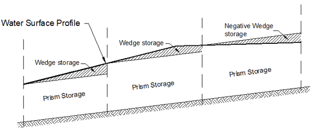
The Muskingum routing method is similar to the Modified Puls method in that a conservation of mass approach is used to route flow through the stream reach. However, the Muskingum method accounts for “looped” storage vs. outflow relationships that commonly exist in most rivers (i.e., hysteresis). This can simulate the commonly observed increased channel storage during the rising side and decreased channel storage during the falling side of a passing flood wave. To do so, the total storage in a reach is conceptualized as the sum of prism (i.e., rectangle) and wedge (i.e., triangle) storage, as shown in the following figure. During rising stages on the leading edge of a flood wave, wedge storage is positive and added to the prism storage. Conversely, during falling stages on the receding side of a flood wave, wedge storage is negative and subtracted from the prism storage. Through the inclusion of a travel time for the reach and a weighting between the influence of inflow and outflow, it is possible to approximate attenuation.

This method begins with the following form of the continuity equation:

1)	$\begin{array}{l}\displaystyle \overline{I_{t}}-\overline{O_{t}}=\frac{\Delta S_{t}}{\Delta t}\end{array}$

where $\begin{array}{l}\overline{I_{t}}\end{array}$ = average upstream flow (inflow to reach) during a period $\begin{array}{l}\Delta t\end{array}$ ; $\begin{array}{l}\overline{O_t}\end{array}$ = average downstream flow (outflow from reach) during the same period; and $\begin{array}{l}\Delta S_t\end{array}$ = change in storage in the reach during the period. Using a finite difference approximation and rearrangement yields:

2)	$\begin{array}{l}\displaystyle \left(\frac{I_{t-1}+I_{t}}{2}\right)-\left(\frac{O_{t-1}+O_{t}}{2}\right)=\left(\frac{S_{t}-S_{t-1}}{\Delta t}\right)\end{array}$

where I_t_-1 and I_t = inflow to the reach at times t-1 and t, respectively, O_t_-1 and O_t = outflow from the reach at times t-1 and t, respectively, and S_t_-1 and S_t = storage within the reach at times t-1 and t, respectively.

The volume of prism storage is the outflow rate, O, multiplied by the travel time through the reach, K. The volume of wedge storage is a weighted difference between inflow and outflow multiplied by the travel time K. Thus, the Muskingum method defines total storage as:

3)	$\begin{array}{l}\displaystyle S_{t}=K O_{t}+K X\left(I_{t}-O_{t}\right)\end{array}$

Further simplification yields:

4)	$\begin{array}{l}\displaystyle S_{t}=K O_{t}+K X\left(I_{t}-O_{t}\right)=K\left[X I_{t}+(1-X) O_{t}\right]\end{array}$

where K = travel time of the flood wave through routing reach; and X = dimensionless weight (0 $\begin{array}{l}\mathrm{\leq}\end{array}$ X $\begin{array}{l}\mathrm{\leq}\end{array}$ 0.5).

The quantity $\begin{array}{l}X\left(I_{t}-O_{t}\right)=K\left[X I_{t}+(1-X) O_{t}]\end{array}$ is a weighted discharge. If storage in the channel is controlled by downstream conditions, such that storage and outflow are highly correlated, then X = 0.0. In that case, Equation 4 resolves to a linear reservoir model:

5)	$\begin{array}{l}\displaystyle S_{t}=K O\end{array}$

If X = 0.5, equal weight is given to inflow and outflow, and the result is a uniformly progressive wave that does not attenuate as it moves through the reach.

If Equation 2 is substituted into Equation 4 and the result is rearranged to isolate the unknown values at time t, the result is:

6)	$\begin{array}{l}\displaystyle O_{t}=\left(\frac{\Delta t-2 K X}{2 K(1-X)+\Delta t}\right) I_{t}+\left(\frac{\Delta t+2 K X}{2 K(1-X)+\Delta t}\right) I_{t-1}+\left(\frac{2 K(1-X)-\Delta t}{2 K(1-X)+\Delta t}\right) O_{t-1}\end{array}$

HEC-HMS solves Equation 6 recursively to compute O_t given inflow (I_t and I_t_-1), an initial condition (O_t₌₀), K, and X.

Required Parameters

Parameters that are required to utilize this method within HEC-HMS include the initial condition, K [hours], X, and the number of subreaches. Two options for specifying the initial condition are included: outflow equals inflow and specified discharge [ft³/sec or m³/sec]. The first option assumes that the initial outflow is the same as the initial inflow to the reach from the upstream elements which is equivalent to the assumption of a steady-state initial condition. The second option is most appropriate when there is observed streamflow data at the end of the reach. In either case, the initial storage will be computed from the first inflow to the reach and corresponding storage vs. discharge function.

K is equivalent to the travel time through the reach. Initial estimates of this parameter can be made using observed streamflow data or through approximations of flood wave celerity. One such approximation is Seddon’s Law (Ponce, 1983):

7)	$\begin{array}{l}\displaystyle c=\frac{1}{B} \frac{d Q}{d y}\end{array}$

where c = flood wave celerity [ft/s or m/s], B = top width of the water surface [ft or m], and dQ/dy = slope of the discharge vs. stage relationship (i.e. rating curve). K can then be estimated using:

8)	$\begin{array}{l}\displaystyle K=\frac{L}{c}\end{array}$

where L = length of the reach [ft or m].

X is a dimensionless coefficient that lacks a strong physical meaning. This parameter must range between 0.0 (maximum attenuation) and 0.5 (no attenuation). For most stream reaches, an intermediate value is found through calibration.

The specified number of subreaches affects attenuation. One subreach results in the maximum amount of attenuation and increasing the number of subreaches approaches zero attenuation. For an idealized channel, the travel time through a subreach should be approximately equal to the simulation time step. An initial estimate of this parameter can be obtained by dividing the actual reach length by the product of the wave celerity and the simulation time step. For natural channels that vary in cross-section dimension, slope, and storage, the number of subreaches can be treated as a calibration parameter. The number of subreaches may be used to introduce numerical attenuation which can be used to better represent the movement of flood waves through the natural system.

A tutorial describing an example application of this loss method, including parameter estimation and calibration, can be found here: Applying the Muskingum Routing Method.