Post-Wildfire Hydrology Modeling with Green & Ampt Loss Method using Sorptivity

Last Modified: 2024-12-23 09:56:17.12

This tutorial demonstrates a process to configure and calibrate an HEC-HMS model for pre and post wildfire modeling.

Software Version

HEC-HMS version 4.13 was used to develop this tutorial. 

Project Files

Download the initial project files here:

Arroyo_Seco_Sorptivity_Initial.7z

Introduction

This tutorial guides you through the process of setting up an HEC-HMS post-wildfire hydrology model, using the calibrated pre-wildfire model for the Arroyo Seco Watershed in Los Angeles County. The Arroyo Seco, a tributary of the Los Angeles River, originates in the San Gabriel Mountains. In August 2009, the watershed was significantly impacted by the Station Fire, which burned 65,000 hectares in the Angeles National Forest, including approximately 95% of the Arroyo Seco Watershed.

This procedure is designed for situations requiring rapid model development, with limited calibration. The resulting model will estimate peak discharges, which can later be used to calculate debris yields and identify areas at the highest risk of flooding. A final copy of the project is provided at the end of this tutorial.

An HEC-HMS pre-wildfire hydrology model for the Arroyo Seco Watershed has already been prepared for you. A Digital Elevation Model (DEM) was integrated into the project and used to delineate the watershed in HEC-HMS. Watershed delineation is easily performed in HEC-HMS when a projected terrain file is provided, and the software can automatically extract watershed characteristics once the basin is delineated.

For more information on pre-wildfire hydrology models using the Green and Ampt (G&A) loss method and the SCS-CN method, refer to the following resources:

1. Applying the Green and Ampt Loss Method

2. Pre & Post Wildfire Hydrology Modeling Procedure with SCS-CN Loss Method

In this workshop, you will prepare the post-fire hydrology model using the calibrated pre-wildfire model, applying the G&A loss method in HEC-HMS with Sorptivity.

Post-Fire Model Setup

1. Create post-fire basin models by adjusting the Moisture Deficit, Sorptivity, and Hydraulic Conductivity based on the below guidance table to reflect post-fire conditions.
2. For the Arroyo Seco watershed model, three pre-fire input parameter values must be converted to post-fire values using burned area emergency response (BAER) soil burn severity maps and guidance table developed based on the Walnut Gulch rainfall simulator dataset (Polyakov et al., 2018). This approach requires the following steps:
   1. Determine the percentage of all burn area including (low, moderate, and high burn) for each subbasin.
      1. Click the link below for detailed steps on calculating burn severity percentages.

         1. Watershed Burn Severity Calculation Procedure

   2. A guidance table was developed for the modified G&A loss method with the sorptivity and wetting front suction value by Jay Pak et al., using the Walnut Gulch rainfall simulator dataset. This table is based on the calibration results from 68 pre- and post-fire rainfall simulator datasets (DOI: https://doi.org/10.15482/USDA.ADC/1358583) under wet conditions. This guidance table was used to determine the appropriate initial moisture deficit, sorptivity, wetting front suction, and hydraulic conductivity to apply to each subbasin to compute the post-fire input parameters.
      

      Post-Fire Parameters	1 st Year after Fire Parameter Range For G&A Loss Method (Aid & Semi-Arid Area & Wet Condition)
      	Min	1Q Percentile	Median	3Q Percentile	Max
      Moisture Deficit Values	0.12	0.08	0.07	0.021	0.08
      Wetting Front Suction Multiplier	0.942 * (Pre-Fire Moisture Deficit Value/Post-Fire Moisture Deficit Value) 2	0.912 * (Pre-Fire Moisture Deficit Value/Post-Fire Moisture Deficit Value) 2	0.912 * (Pre-Fire Moisture Deficit Value/Post-Fire Moisture Deficit Value) 2	0.842 * (Pre-Fire Moisture Deficit Value/Post-Fire Moisture Deficit Value) 2	0.752 * (Pre-Fire Moisture Deficit Value/Post-Fire Moisture Deficit Value) 2
      Sorptivity Multiplier	0.94*(Pre-Fire Moisture Deficit Value/Post-Fire Moisture Deficit Value)	0.91*(Pre-Fire Moisture Deficit Value/Post-Fire Moisture Deficit Value)	0.91*(Pre-Fire Moisture Deficit Value/Post-Fire Moisture Deficit Value)	0.84*(Pre-Fire Moisture Deficit Value/Post-Fire Moisture Deficit Value)	0.75*(Pre-Fire Moisture Deficit Value/Post-Fire Moisture Deficit Value)
      Hydraulic Conductivity Multiplier	1.91	1.23	0.87	0.46	0.14

      
      
      
3. Computing the initial three parameter values for every subbasin by hand is unrealistic, so a spreadsheet was developed to automate the process.
   1. Use the "Post-Fire_Parameter_Values_GreenAmpt" spreadsheet in the data folder.
   2. Copy the Hydraulic Conductivity, Sorptivity, and Initial Deficit from the pre-fire calibrated basin model (01_Pre_2006_01_ReC_S) using the glover editor, and paste them into the 'G&A_Sorptivity' tab of this spreadsheet. The Burned Area Percentage was provided in spreadsheet.   
      
   3. The remainder of the spreadsheet will auto-populate based on the percentage of burned area and the guidance table values for post-fire Conductivity, Sorptivity, and Initial Deficit, categorized as minimum, median, and maximum.
4. Create post-fire basin models for each category as minimum, median, and maximum.
   1. Copy the pre-fire basin models (01_Pre_2006_ReC_S) by right clicking on the pre-fire basin models and selecting Create Copy... for three categories as 01_PreP2006_ReC_S_Max, 01_Pre_2006_ReC_S_Median, and 01_Pre_2006_ReC_S_Min.
   2. Using the global editor, update the post-fire Conductivity, Sorptivity, and Initial Deficit values for the three basin models (01_Pre_2006_ReC_S_Max, 01_Pre_2006_ReC_S_Median, and 01_Pre_2006_ReC_S_Min) with the computed values from the spreadsheet.
   3. Create and Compute a Simulation Run with the existing Meteorologic Model (LA Rain Gages_Hourly_Adj) and Control Specifications (02_Post_2010_01_01).
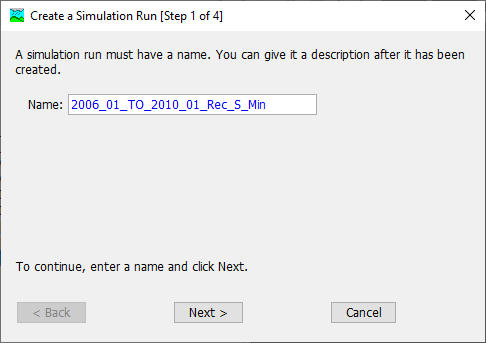
      1. Click on the Compute menu and select the Create Compute | Simulation Run option. A wizard window will open to guide you in creating a new simulation run. In the first step enter name 2006_01_TO_2010_01_Rec_S_Min.
         
         1. In second step, choose the 01_Pre_2006_01_Rec_S_Min basin model. In third step, choose the LA Rain Gages_Hourly_Adj meteorologic model. In Step 4, choose the 02_Post_2010_01_01 control specifications. Press the Finish button to complete the process of creating a simulation run.

         2. A simulation run must be selected before it can be computed. The tool bar includes a selection list that shows all of the simulation runs that have been created in the project. Click on the selection list and choose RUN: 2006_01_TO_2010_Rec_S_Min. Once a simulation run has been selected, click on the Compute button  immediately to the right of the selection list to perform the compute. The tool bar button has an icon of a raindrop whenever a simulation run is selected. A compute progress window will open to show the advancement of the simulation. The simulation may abort if errors are encountered. If this happens, read the messages and fix any problems; then compute the simulation run again. Close the progress window when the run computes successfully.
            

   4. Create and Compute a Simulation Run with the existing Meteorologic Model (LA Rain Gages_Hourly_Adj) and Control Specifications (02_Post_2010_01_01) for remaining two basin models (01_Pre_2006_ReC_S_Max, and 01_Pre_2006_ReC_S_Median) by repeating the previous step i.

Viewing Post-Wildfire Hydrology Results

In the HEC-HMS Results tab, users can view three flow results from different simulation runs. Each element displays typical hydrologic outputs. By selecting options like Graph, Summary Table, or Time-Series Table under each element, only the relevant outputs are displayed.   

1. To view post-wildfire hydrology simulation results at the outlet, follow these steps:
   1. Go to the Results tab and select the ArroyoSeco_USGS sink element.
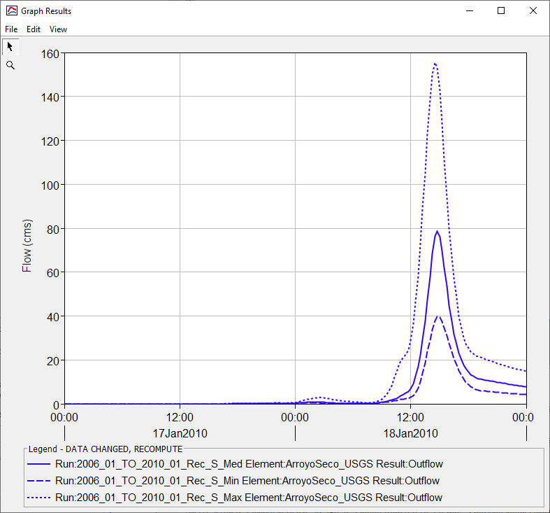
   2. Hold the 'Ctrl' key and click on the Outflow results from the three different simulation runs: RUN: 2006_01_TO_2010_Rec_S_Min, RUN: 2006_01_TO_2010_Rec_S_Med, and RUN: 2006_01_TO_2010_Rec_S_Max. These runs represent the hydrographs under three post-fire flow scenarios for minimum, median, and maximum conditions.
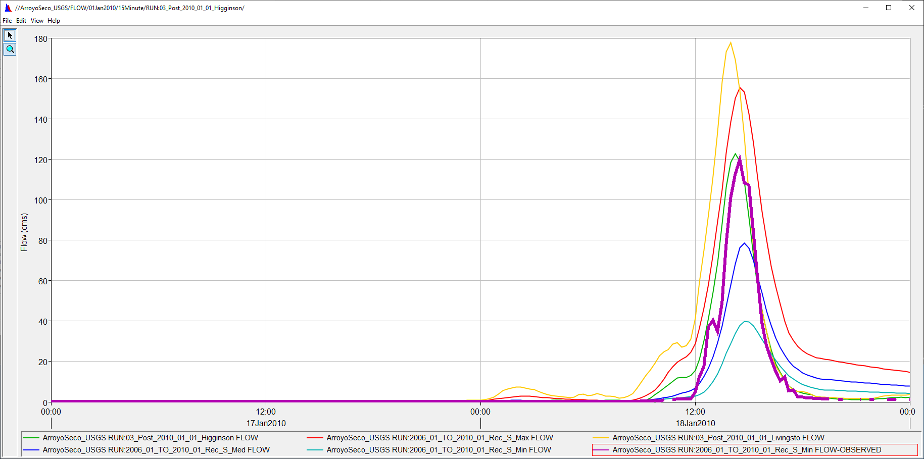
   3. The post-fire flow results are displayed with a range between minimum, median, and maximum values. The graph below compares the estimated post-fire hydrographs for the minimum, median, and maximum scenarios, highlighting the uncertainty range between the minimum and maximum values.
       

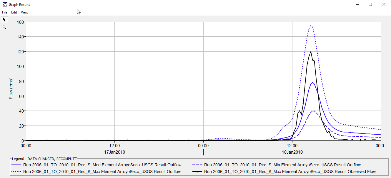
Question 1: Do you think the Green and Ampt method, along with the guidance table, provides a reasonable estimate for future post-wildfire outflow runoff?

Question 2: Do you believe the Green and Ampt method, incorporating sorptivity and the guidance table, could serve as an alternative to the SCS-CN method for post-fire hydrology analysis?

Create the Ensemble Analysis and Compute

Each of the three simulation runs were computed as minimum, median, and maximum by showing degrees of uncertainty. However, as an alternative you can use an quilted in ensemble analysis tool in HEC-HMS. An ensemble analysis can be used to aggregate the predictions of each base model into one general prediction. If the base models are diverse and independent of each other, the prediction error of the base models decreases when using the ensemble approach. The following steps show you how to create an ensemble analysis model that includes each of the base simulation run models.

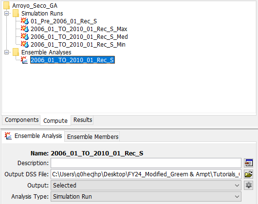
1. From the top menu bar, select Compute | Ensemble Analysis Manager.
   
2. Select New... and name the analysis 2006_01_TO_2010_01_Rec_S. Select Simulation Run as the analysis type and then select Next. 
   
3. All of the simulation runs that have been previously created are available for selecting as part of this ensemble analysis. Select them all by moving them from the left window pane to the right window pane. Select Next and then Finish.
   

4. Now that the ensemble analysis has been created, we can select and further refine it by selecting the Compute tab of the Watershed Explorer. 
   

   

   Note:

   Depending on the detail and number of simulation runs that are included within an ensemble analysis, the file size of the HEC-HMS project can quickly balloon. An important way to keep computation time and file sizes more manageable is to only generate the results output that you as the user are interested in. 

   To select the time-series results output that you wish to generate during a compute, select the output gear icon. 
   
   For this analysis, we aim to compute all available time-series results for ArroyoSeco_USGS, including both Outflow and Cumulative Outflow, with a 1-hour output interval. Click Save and then Close to exit the window. 
   
   

   
   

   Note:

   When the above output control table is populated, all of the ensemble analysis members are iterated over. Only the elements and time-series that are available in ALL of the members will be available for selection within the table. If, for example, an element is present in some of the members (simulation runs) but not all of them, it will not be available for analyzing within the ensemble analysis compute.

   If needed, simulation runs can be removed and/or added to the ensemble analysis via the table located on the Ensemble Members tab. We wish to include two of the previously selected simulation runs so no further refinement is necessary.
   

5. Finally, let's compute the Ensemble Analysis. Select Ensemble: 2006_01_TO_2010_01_Rec_S in the compute dropdown and then click the Ensemble Analysis icon to begin the compute.
   
   During the Ensemble Analysis compute, each of the base simulation runs will first be computed and then the final ensemble results will be aggregated.
   

View the Ensemble Analysis Results

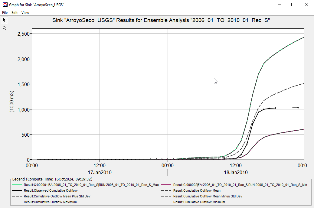
1. The Ensemble Analysis results can be accessed in the Watershed Explorer via the Results tab. Results should only be available for the elements and time-series that you selected earlier. Expand the results for the ArroyoSeco_USGS sink element. 
   
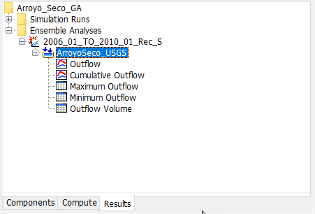
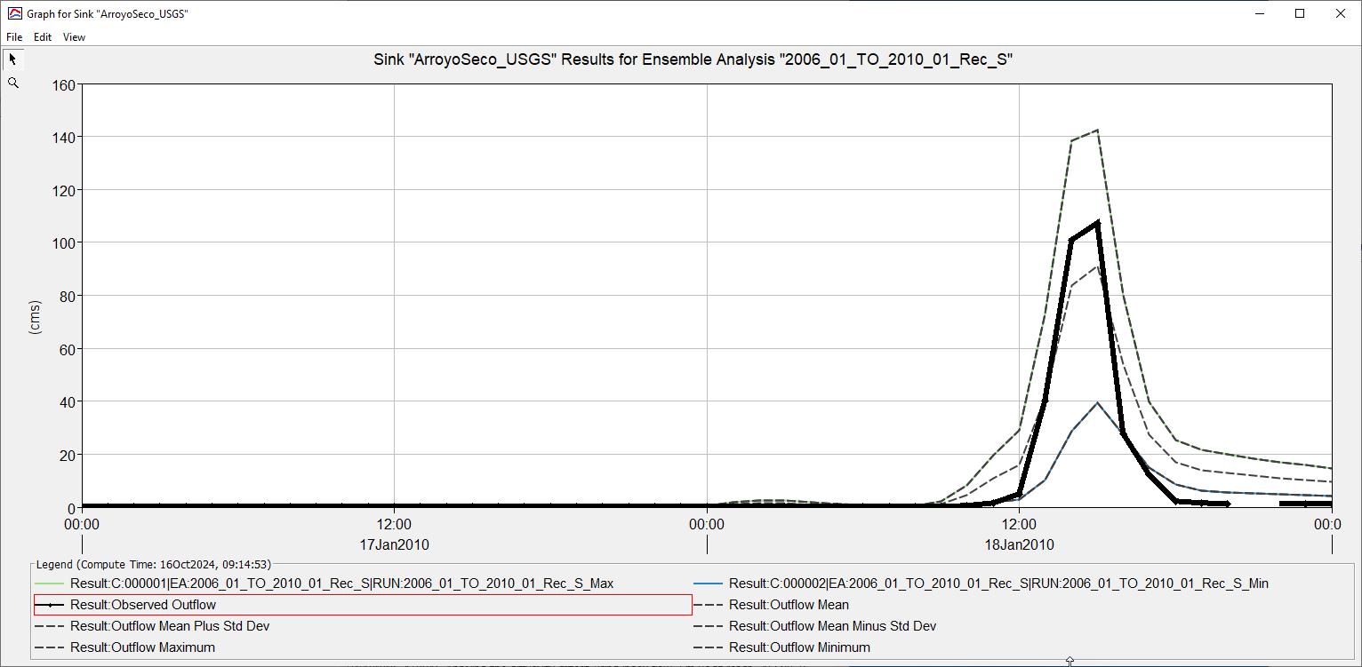
2. Select the Outflow plot node to see a time-series plot of the results. In addition to seeing the traces from each of the two simulation runs, you will also notice aggregated time-series results including Outflow Maximum, Minimum, Mean, and +/- One Standard Deviation. Selecting an individual time-series within the legend will bolden it in the plot for easier visualization. 
   

Question 3: Select the Cumulative Outflow plot node to view the results. At the end of the two day simulated time period, wat is the mean cumulative outflow volume?

Project Files

Download the final project files here:

Arroyo_Seco_Sorptivity_Final.7z