Download PDF
Download page Calibrate the Deficit & Constant Basin Model for a Single Water Year.
Calibrate the Deficit & Constant Basin Model for a Single Water Year
Return to Introduction to Calibrating a Continuous Simulation Model
Last Modified: 2024-09-03 19:32:54.442
HEC-HMS Version
HEC-HMS version 4.12 was used to create this tutorial. You will need to use HEC-HMS version 4.12, or newer, to open the project files.

Step 1: Initialize the Model
Prior to calibrating, a model must be initialized with parameter estimates. Some parameters can be estimated provided a physical description of the watershed. Others can be estimated given results from previous studies or regional studies that cover the basin area.
- Open the EF Russian DC 2005 basin model.
The Clark transform Time of Concentration (Tc) parameter (the time it takes for runoff to travel from the most distant point in the watershed to the outlet) was estimated using the TR-55 method (SCS, 1986). The TR-55 method uses physical basin parameters such as length and slope provided from GIS analysis. The Clark Storage Coefficient (R) is a calibration parameter that affects the shape of the runoff hydrograph, meaning this parameter is set using measured rainfall-runoff data. Initial estimates for Tc and R were based on calibrated values from a previous event base study. Initial Clark transform parameters are presented in Figure 1.
Canopy and surface Max Storage loss parameters were initialized based on values provided in literature. The initial condition of the surface should be specified as the percentage of the surface storage that is full of water at the beginning of the simulation. The Initial Storage parameter for both canopy and surface loss methods was set to 0 because the simulation begins during an extended dry period for the basin. Initial canopy loss parameters are presented in Figure 2. Initial surface loss parameters are presented in Figure 3. 

Deficit and constant soil loss parameters Maximum Deficit and Constant Rate were estimated based on a Soil Survey Geographic (SSURGO) database (USDA 2015) analysis in GIS. Percent Impervious was estimated from a land use data set analysis in GIS. Initial subbasin loss parameters are presented in Figure 4. Select the "Loss" tab in the component editor for subbasin "EF Russian 20." The Initial Deficit indicates the amount of water that is required to saturate the soil layer to the maximum storage.- Set the Initial Deficit to 10.9 inches (assume the simulation begins during an extended dry period and all soil moisture has been depleted).

- Linear reservoir baseflow parameters are set by a graphically fitting the recession limb of the computed runoff hydrograph with the observed flow. The groundwater storage coefficient is the time constant for the linear reservoir in each layer. Since it is measured in hours, it gives a sense of the response time of the subbasin. The GW 1 Coefficient and GW 2 Coefficient are proportionally larger than the time of concentration for the basin. The number of GW 1 Reservoirs and GW 2 Reservoirs were both set to 1. The GW 1 Initial and GW 2 Initial parameters for the surface loss method were set to 0 because the simulation begins during an extended dry period for the basin. Initial subbasin baseflow parameters are presented in Figure 5.

- A simulation run named WY 2005 DC has been created that incorporates the basin model EF Russian DC 2005. Run the simulation WY 2005 DC.
- View the computed vs observed hydrographs at the Calpella Gage junction by browsing the Results tab in the watershed explorer, expanding the Calpella Gage node and clicking "Graph" (Figure 6). A plot of computed vs observed flow will be generated for the water year (Figure 7).


Step 2: Calibrate the Early Wet-Season
- With the initial model run complete, the first focus area for calibration is the early wet-season events. Notice for the first major observed event, the computed results fail to reproduce a runoff response (Figure 8).

This indicates that the soil layer absorbs all of the precipitation that fell on the subbasin. Because the soil layer needs to be saturated to generate a significant runoff response the soil layer capacity, or, Maximum Deficit, must be reduced. - HEC-HMS provides soil moisture records as output to a simulation run. The best way to visualize soil moisture is by selecting the following results simultaneously (hold ctrl while selecting results). On the Results tab in the watershed explorer, under the EF Russian 20 node, select "Precipitation" and "Moisture Deficit" results, under the Calpella Gage node select "Outflow" and "Observed Flow" results (Figure 9). With the results selected in the watershed explorer click the View Graph
 button in HEC-HMS to view results (Figure 10).

The soil layer should reach a Deficit = 0 inches during the first major observed runoff event. As a start for calibration, the Maximum Deficit can be reduced by approximately the deficit at the beginning of the 7-9 December 2004 event (Figure 11). Note: the Initial Deficit will likely need to change as well as it cannot exceed the Maximum Deficit. At the end of a long dry period the Initial Deficit should be equal to or be close to the Maximum Deficit.
- Adjust the Maximum Deficit and Initial Deficit. Re-run the model until the computed hydrograph reproduces the observed for the first event (Figure 12).

Step 3: Calibrate Baseflow
The next focus area for calibration is the recession limb of hydrographs. The recession limb is important when considering the overall Nash-Sutcliffe Efficiency and the distribution of volume. The recession limb of hydrographs are most sensitive to baseflow parameters GW 1 Coefficient, GW 2 Coefficient, GW 1 Reservoirs, and GW 2 Reservoirs. In this case, the GW 1 Coefficient has the most influence on the recession limb calibration. Adjust the GW 1 Coefficient and re-run the model until the computed recession limbs reproduce the observed (Figure 13). Remember that GW Coefficients correlate to the groundwater response time and GW Reservoirs correlates to groundwater attenuation. Scroll through the results at Calpella Gage to graphically evaluate fit for recession hydrograph limbs (Figure 13).
To assist with the baseflow calibration, users can select in the Results tab for ER Russian 20 the Baseflow Layer 1 and Baseflow Layer 2.
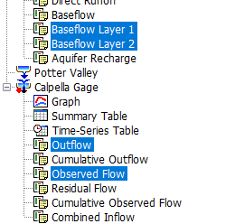
Selecting these outputs will show the baseflow for each layer and help with deciding which layer to focus on adjusting.
Step 4: Calibrate peak flows
Peak flows are most sensitive to the Constant Rate loss parameter. The Constant Rate represents the infiltration capacity of the soil. Think about how adjusting the Constant Rate parameter might affect peak runoff. Adjust the Constant Rate and re-run the model until the computed peaks reproduce the observed (Figure 14).
Step 5: Quantify Results
Once calibrated, view summary results (Figure 15) for the Calpella Gage element. Your results will be slightly different than the results shown below.

Summary results for calibrated "EF Russian 20 DC" Basin for simulation “WY 2005 DC” are presented in the table below. Results may vary.
| Computed | Observed | |
|---|---|---|
| Peak Discharge (CFS) | 6187.4 | 6552.5 |
| Volume (AC-FT) | 231495.6 | 213599.1 |
The Nash-Sutcliffe Efficiency of the calibrated model is ~0.841. Results may vary.
Final parameters of the calibrated model are presented in the table below. Results may vary.
Element | Parameter | Value |
Canopy | Crop Coefficient | 0.3 |
Loss | Initial Deficit (IN) | 6.5 |
Maximum Deficit (IN) | 6.5 | |
Constant Rate (IN/HR) | 0.125 | |
Transform | Time of Concentration (HR) | 5.5 |
Storage Coefficient (HR) | 4.5 | |
Baseflow | GW 1 Coefficient (HR) | 28 |
GW 1 Reservoirs | 1 | |
GW 2 Coefficient (HR) | 400 | |
GW 2 Reservoirs | 1 |
Continue to Calibrate the Soil Moisture Accounting Basin Model for a Single Water Year