You will be inputting initial values to each model parameter. These initial values have already been calculated and computed for you. You can review how these initial values were estimated from previous tutorials.
Initial parameters
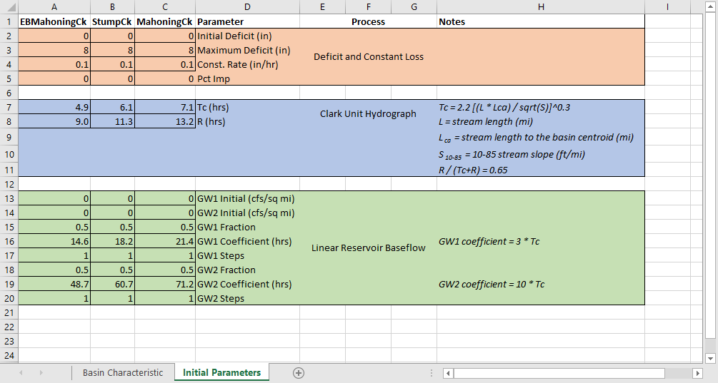
Open "Punx_Parameters.xlsx" spreadsheet and navigate to the Initial Parameters tab.
Open the Punx HMS project
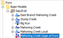
Select the Basin Model Sep2018
Populate the Deficit and Constant Loss
Select East Branch Mahoning Creek subbasin element. In the Component Editor navigate to the Loss tab
Enter in the loss values from the Excel spreadsheet
Repeat for Stump Creek and Mahoning Creek Local
Hint
Use global editors to speed up parameter entry. To access the global editor for subbasin loss, go to Parameters | Loss | Deficit and Constant
Populate the Clark Unit Hydrograph
Select East Branch Mahoning Creek subbasin element. In the Component Editor navigate to the Transform tab
Enter in the transform values from the Excel spreadsheet
Repeat for Stump Creek and Mahoning Creek Local
Populate the Linear Reservoir Baseflow
Select East Branch Mahoning Creek subbasin element. In the Component Editor navigate to the Baseflow tab
Enter in the baseflow values from the Excel spreadsheet
Repeat for Stump Creek and Mahoning Creek Local
Add observed hydrograph to Mahoning Creek Gage at Punx. The observed dataset has already been prepared for you under Time-Series Data |Discharge Gages | Punxsutawney
In the Basin Model Sep2018, select the Mahoning Creek Gage at Punx element
In the Component Editor, navigate to the Options tab and select Punxsutawney for Observed Flow.
Create a simulation run.
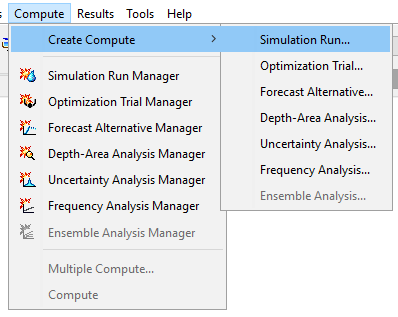
Navigate to the Compute tab
Click on Compute | Create Compute | Simulation Run in the File Menu
Name your simulation Sep2018. Select your Basin Model, Meteorological Model, and Control Specifications in the Create a Simulation Run Wizard
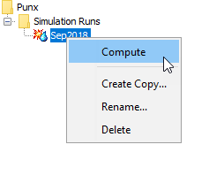
Right click Sep2018 | Compute
Review your results
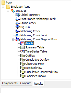
Navigate to Results tab.
Click on Sep2018 and expand the Mahoning Creek Gage at Punx Element. Plot the Graph and Summary Table to view results