Download PDF
Download page Calibrate a Basin Model to Event 1.
Calibrate a Basin Model to Event 1
Last Modified: 2023-11-17 09:53:31.757
Software Version
HEC-HMS version 4.12 beta 3 was used to create this example. You can open the example project with HEC-HMS 4.12 or a newer version.
Download the project file with initial parameters populated from the Populate Initial Parameters workshop (make sure to use the final file at the end of the workshop).
Overview
We will start adjusting our parameters to better match the observed hydrograph. The tutorial below will walk you through one way of systematically calibrating your model to match the observed hydrograph. We will work through adjusting the losses, then move onto adjusting your unit hydrograph parameters, then lastly your baseflow parameters. Other hydrologists and engineers may have their own calibration techniques.
Keep in mind that calibration is an iterative process! Just because one parameter looks good after your first adjustment doesn't mean you won't need to go back and refine the parameter value again; however, calibration should be more than just adjusting parameters to best match a curve. It is also important to have a good understanding of the watershed hydrology and know what are the reasonable ranges for model parameters. If your watershed consists of mainly sandy, well draining soils, it wouldn't make much sense to set your loss rates to 0 inches per hour just so you can match your hydrograph volume. Have a reason to why you are making your adjustment. Parameter values should make sense to the watershed and the types of events you are modeling. This will allow you to have confidence in your model results and defend your modeling results when you're able to explain the why behind the values. When you start needing to adjust your model beyond reasonable limits, this may suggest issues with your model boundary conditions, your model set up, or something more fundamental about your basin that isn't being captured.
Adjust Deficit and Constant Loss Method
- Review Results from initial simulation
- Using the Punx model developed from the Populate Initial Parameters (or using the workshop project provided), review your simulated results at element Mahoning Creek Gage at Punx.
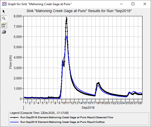
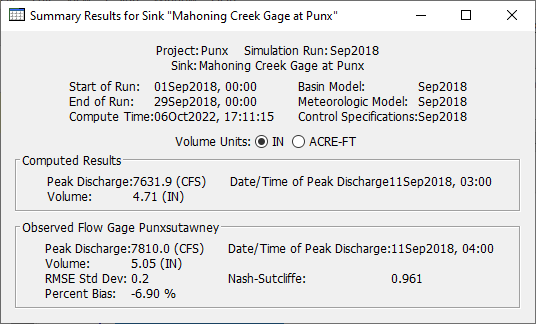
- Open the Graph and Summary Table. Keep the graph and summary results open while you are calibrating parameters. This will help you to observe how your parameter changes affect your simulated results.
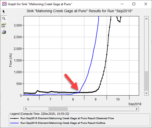
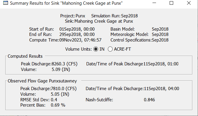
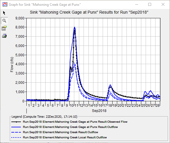
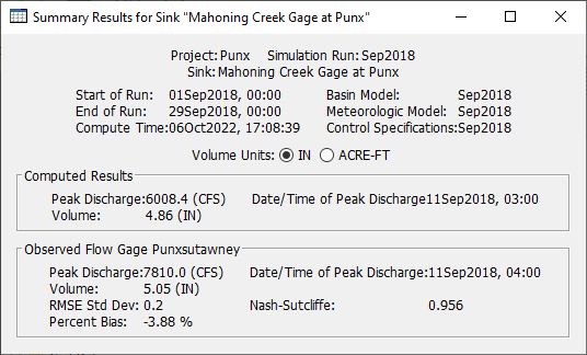
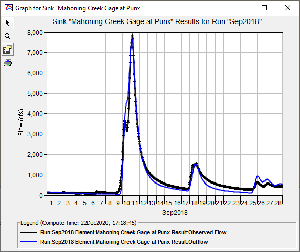
By visually inspecting the hydrograph, you can easily see the simulated flow has a higher volume and peak value than the observed hydrograph. You can confirm the high volume by checking the differences in the Summary Results table (compare Compute Volume to the Observed Volume). We'll start the calibration by adjusting the Deficit and Constant Loss rate. - Open the global editor for the Deficit and Constant Method by selecting on the File Menu Parameters | Loss | Deficit and Constant.
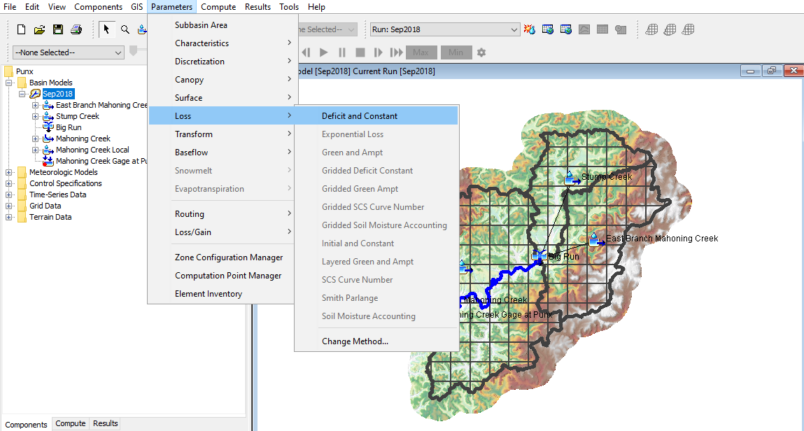
The Deficit and Constant global editor should appear. Make sure you have your basin model Sep2018 selected before opening the editor.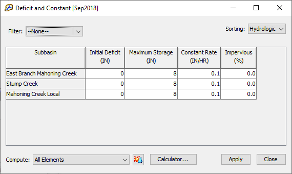
- Notice that the rising limb of the computed hydrograph begins on September 8, about a day earlier than the rising limb for the observed hydrograph.
We currently have initial loss set at "0". This means there is no initial deficit of water that needs to be filled prior to runoff initiation other than the constant loss. It is unlikely for the ground storage to be fully saturated given the little rainfall from the prior 8 days. Adjust the initial deficit to the point where the observed hydrograph begins. In the figure below, initial loss was changed to 1.5 inches for all subbasins. Re-run your simulation and compare the results.

Adjust Clark Unit Hydrograph
- Open the global editor for the Clark Unit Hydrograph method
- Select the File Menu Parameters | Transform | Clark Unit Hydrograph. The Clark Unit Hydrograph global editor should appear. Make sure you have your basin model Sep2018 selected before opening the editor.
Compare your simulated hydrograph peak to the observed flow. The simulated peak occurs earlier than the observed peak. Which parameter do you think you should adjust?
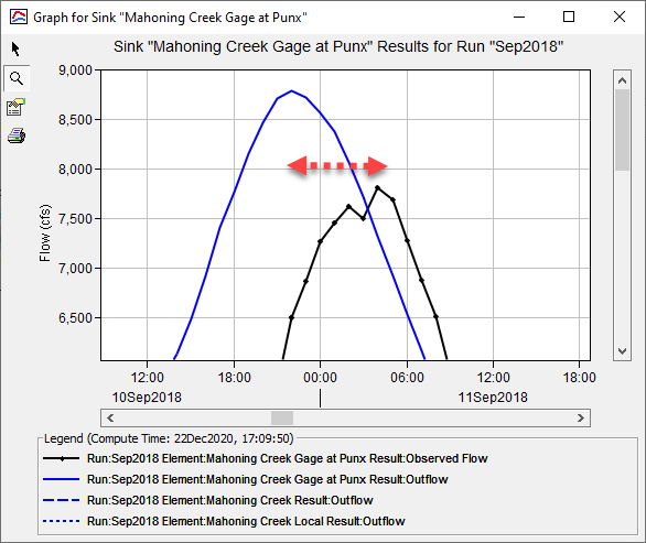
Time of Concentration! Try adjusting your time of concentration until you get a good match to the timing. Since you have three subbasins that contribute to this outlet, consider adjusting all the Tc values by the same factor. Adjusting models by the same factor can be a useful technique when you do not have additional information to suggest otherwise. If you are fortunate to have another flow gage or highwater mark on an upstream tributary, this information should be used to make unique subbasin parameter adjustments. In the figure below, the Tc was increased by a factor of 2.2 for all subbasins.

The storage coefficient has a large effect on the shape of the hydrograph. The simulated hydrograph appears to reasonably match the shape of the observed hydrograph but could be adjusted slightly. Change the storage coefficient by a factor of 1.2 for all three subbasins.
Adjust Linear Reservoir Baseflow
- Open the global editor for the Linear Reservoir Baseflow Method
- Select the File Menu Parameters | Baseflow | Linear Reservoir Baseflow. The Linear Reservoir Baseflow global editor should appear. Make sure you have your basin model Sep2018 selected before opening the editor.
Compare your simulated hydrograph recession limb to the observed recession.
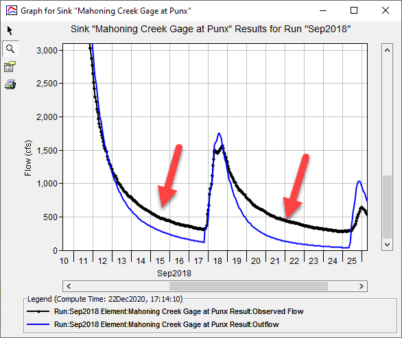
It appears that the baseflow could be extended out further past the inflection point. What parameter within the Linear Baseflow Method would you adjust?GW 1 and GW 2 Coefficients! These coefficients govern the travel time of your interflow (GW 1) and deeper baseflow (GW 2). Triple both your GW 1 and GW 2 coefficients for all subbasins and review results. Iterate as necessary.
Review results
At this point, we've made initial adjustments to the simulated hydrographs. You may have noticed that adjustments for one parameter could affected another part of the hydrograph you did not intend to change. For example, while increasing the GW 1 & 2 coefficients for baseflow, the hydrograph peak was reduced. We may want to revisit our loss rate parameters and see if reducing our constant loss rate might help. Unless there is a compelling reason, avoid making drastic adjustments to one parameter to compensate for an adjustment to another. Continue to keep in mind reasonable parameter ranges as you make your adjustments and that the parameters you are selecting make sense for your basin.
If you haven't already noticed, your Summary Results provides useful statistical metrics to assist in calibration. A useful metric commonly used is the Nash-Sutcliffe Efficiency (NSE), which measures the predictive skill of a hydrologic model. A value of "1" means the simulated values can perfectly predict the observed where there is no estimation error variance, while a value of "0" means the estimation error variance is equal to the error variance in the observed data. As you were making adjustments to your model, you may have noticed the NSE increasing, suggesting that your model predictions are improving. Moriasi, et. al, 2007 developed a performance rating table based on commonly used statistical measures to evaluate model performance.
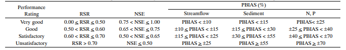
This can be one of several methods to assess model performance. The NSE and the other metrics provided are useful indicators on how your model prediction is performing; however, similar to the issue with curve fitting, the modeler should not focus solely on maximizing the NSE or other single metric. The calibration process should also take into account the needs of the project (i.e. concerned with peak flow, volume, or both) and you're understanding of the watershed through research and analysis.
- Refine parameters
Navigate back to your Deficit and Constant loss rate editor. The Summary Results shows simulated volumes are low. What parameter could we consider adjusting?
Consider reducing your constant loss rate some more. We made changes to the initial deficit initially but didn't make any changes to the constant rate. Change your initial Deficit to 1.8 inches and your constant loss rate to 0.05 inches per hour.
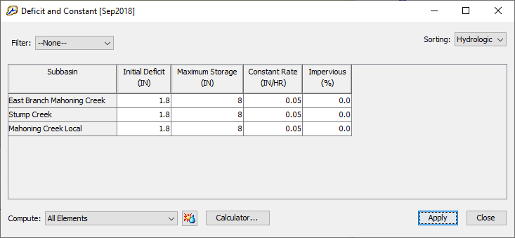
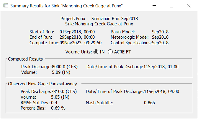
Reducing the constant loss rate helped to better match the hydrograph peak flow. Review your Summary Results. How do the simulated results compare to the observe results?
Simulated results have improved significantly compared to the initial results. The peak timing, peak flow, simulate volume, and NSE values are within a reasonable range.
- Feel free to adjust other parameters and see if you could further improve the simulated results
Download final Project files here
 Event 1 Calibration - solution.zip
Question
Did you make any additional changes to your parameters? What was your final Nash-Sutcliffe Value?
Answers will vary
Why is it important to not just curve fit or maximize NSE?
You want to make sure your model parameters make physical sense and that you're not misrepresenting your watershed basin. For example, you may come across a scenario where increasing your percent impervious will help with increasing runoff volume and your peak flow and therefore get a better match to your observed runoff. But, this wouldn't make any physical sense if there wasn't any evidence of urbanization. If your study was looking for alternatives to reduce peak flow from the basin, your model will be misrepresenting the physical processes driving the peak.
Continue to Calibrate a Basin Model to Event 2