Download PDF
Download page Applying the Frequency Analysis Compute Type.
Applying the Frequency Analysis Compute Type
Last Modified: 2025-08-11 14:57:50.045
Software Version
HEC-HMS version 4.14-beta.1 was used to create this tutorial. You will need to use HEC-HMS version 4.14, or newer, to open the project files.
Suggested Time
This workshop should take approximately 30-min to complete.
Background
In this tutorial, you will learn how to apply the Frequency Analysis compute option which became available in HEC-HMS v4.10. You will 1) use the Frequency Analysis Manager to create a new Frequency Analysis compute. You will then learn how to 2) add ordinates to the new compute, and 3) compare the computed frequency results to an "observed" frequency curve from a separate Bulletin 17C analysis.
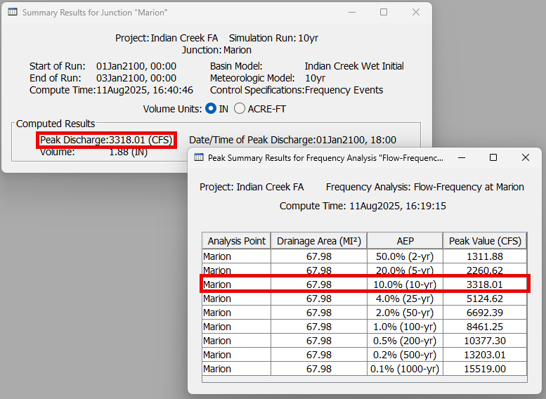
The Frequency Analysis consolidates multiple simulation runs and summarizes their results within a single table. Prior to the addition of the Frequency Analysis compute type, modelers would need to create and run a simulation for each frequency event. Results could only be viewed for the individual simulations. This tutorial demonstrates how the Frequency Analysis compute option removes the need for individual simulation runs, reducing analysis to a single simulation run that provides the results in a single table. This enhancement provides noticeable time savings while also making data management much easier.
In HEC-HMS v4.14, Flow-Frequency curve and Stage-Frequency curve paired data types were added. A Frequency Analysis can be tied to an "observed" frequency curve from either a manual paired data entry in HEC-HMS or directly to DSS output from a Bulletin 17C analysis in HEC-SSP.
Data
The provided watershed–Indian Creek–has been divided into four subbasins, with a computation point at the Marion Junction. The initial watershed has been calibrated to the July 2014 event. The project contains Atlas 14 grids for 24 hour duration 2 year through 1000 year events. Also included are nine hypothetical storm meteorologic models that utilize the Atlas 14 grids. Finally, the Atlas 14 Region 3 Quarter 2 50% time pattern has been added to the model.
Existing simulation runs include a calibration simulation for the July 2014 event, as well as simulation runs for each of the nine frequency events. This initial watershed represents what would be the final results when modeling frequency events prior to the addition of the Frequency Analysis compute type.
Creating a Frequency Analysis compute
The Frequency Analysis compute feature provides a convenient method of combining multiple simulation computes into a single compute while also providing the benefit of consolidating the results of the multiple computes to create a computed frequency curve.
- Click Compute | Frequency Analysis Manager.
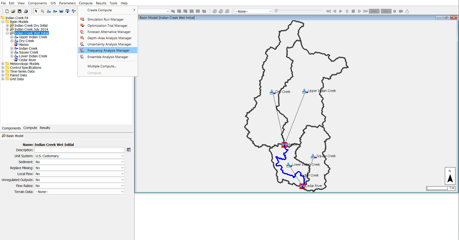
- In the Frequency Analysis Manager, click the New button.
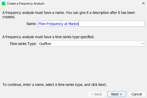
- Name the new Frequency Analysis compute Flow-Frequency at Marion, then click the Next button. Click the Finish button to complete the creation of the new compute type.
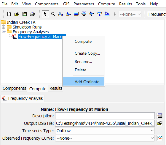
- Navigate to the watershed explorer, Compute tab. A new Frequency Analysis folder has been added to the tree. Expand the folder and right click on Flow-Frequency at Marion, then click Add Ordinate to add the first ordinate.
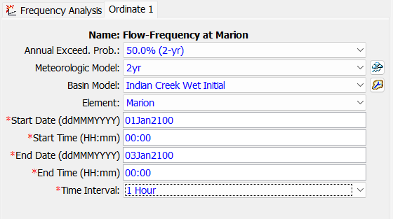
- Fill in the parameters for Ordinate 1 as shown in the figure below. Set the Annual Exceedance Probability to the 50.0% (2-yr) event. This ordinate will use Indian Creek Wet Initial for the Basin Model and the 2yr meteorologic model. Choose Marion as the element. Set the start date to 01Jan2100 and start time to 00:00. Set the end date to 03Jan2100 and end time to 00:00. Finally, the simulation time interval should be set to 1 Hour.
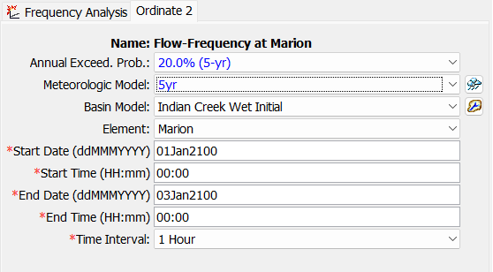
- Create Ordinate 2 by right clicking on Ordinate 1 in the tree and selecting Copy Ordinate. Change the selected Annual Exceedance Probability to the 20.0% (5-yr) event and choose the 5yr Meteorologic Model. The remaining parameters will remain the same as Ordinate 1.
- Create 7 copies of Ordinate 2 (for a total of 9 Ordinates), changing the Annual Exceedance Probability and Meteorologic Model for each ordinate. When finished, you should have ordinates for the 2-yr, 5-yr, 10-yr, 25-yr, 50-yr, 100-yr, 200-yr, 500-yr, and 1000-yr events.
Defining an "observed" frequency curve for a Frequency Analysis
In HEC-HMS version 4.14, Flow-Frequency curve and Stage-Frequency curve paired data types were added to the program. These data types can be associated with a Frequency Analysis in order to compare computed results in HEC-HMS to other "observed" results such as a flow-frequency curve from a Bulletin 17C analysis. First, we will create a Flow-Frequency curve in the project. Then, we will add the curve to the Frequency Analysis as an "Observed Frequency Curve".
- Click Components | Create Component | Paired Data to create a new Paired Data.
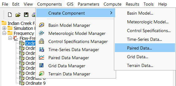
- For Data Type, select Flow-Frequency Curve. Enter Marion B17C for the name.

- Navigate to the watershed explorer, Components tab. Expand the Paired Data folder, and select the Marion B17C paired data node. Flow-Frequency Paired Data can be entered manually or imported from an existing HEC-DSS file. In this case, HEC-SSP was used to perform a Bulletin 17C anlysis at the Marion streamflow gage. A copy of the Bulletin 17C results from HEC-SSP, Marion_B17C.dss, has been placed in the data folder of these workshop project files.
- For Data Source, select Data Storage System (HEC-DSS)
- For DSS Filename, click the folder icon button, navigate to ...\Initial_Indian_Creek_FA\data and select the Marion_B17C.dss file.
- For DSS Pathname, click the pathname icon button, and select the pathname with Marion_B17C in Part B as seen below.
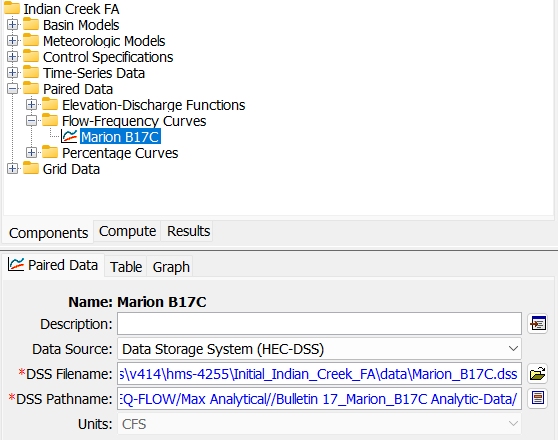
- You may click the Table and Graph tabs to view the imported Flow-Frequency curve from the Bulletin 17C analysis conducted in HEC-SSP.
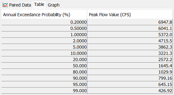
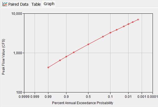
- Now that we have created a Flow-Frequency curve from a Bulletin 17C study, let's reference it in the Frequency Analysis so that we can compare the computed results in HEC-HMS with the Bulletin 17C results.
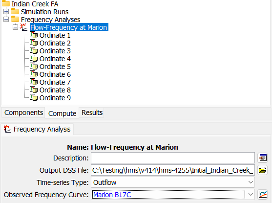
- Navigate to the watershed explorer, Compute tab and select the Flow-Frequency at Marion node. For Observed Frequency Curve, select the Marion B17C paired data object that you just created. Save your project.
Computing a Frequency Analysis and viewing results
- Run the analysis by clicking the Compute button
 in the Compute Control bar. The Compute Progress dialog will open, showing the Ordinates being computed sequentially.
 - View the results of the compute by clicking on the Results tab and expanding the Frequency Analyses | Flow-Frequency at Marion | Marion nodes in the results tree.
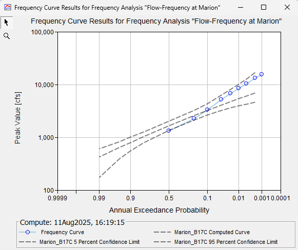
- First, open the Frequency Curve Plot. The Frequency Curve results for Frequency Analysis Flow-Frequency at Marion should appear as shown below. The HEC-HMS computed results for each frequency ordinate are shown in blue and plotted against the "observed" Bulletin 17C results which are shown in grey.
HEC-SSP Output
When a Bulletin 17 C analysis is conducted within HEC-SSP software, the output DSS results contain the computed curve as well as the 5-percent and 95-percent confidence limit curves. Since the paired-data curve in HEC-HMS was created from the HEC-SSP output DSS data, the confidence limit curves are included in this results plot.
Using the Frequency Curve Plot for Calibration
In this workshop example, the computed frequency curve (blue) falls mostly within the observed Bulletin 17C curve (grey) confidence limits. However, the computed ordinates on the frequent end of the curve (2-yr and 5-yr) fall below the observed mean curve whereas the computed ordinates on the rarer end of the curve (25-yr, 50-yr, 100-yr, 200-yr, 500-yr, and 1000-yr) fall above the observed mean curve. The Bulletin 17C results, in this case, contain high levels of uncertainty due to the short record length at the Marion USGS streamflow gage. But, without additional information and context, it might still be prudent to calibrate the model to better match the Bulletin 17C results. In this workshop example, each ordinate is tied to the same basin model. However, for calibration purposes, a unique basin model could be created for each element and key basin parameters could be adjusted until each ordinate better matches the observed mean curve.
- Next, open the Frequency Curve Table. Notice that the Frequency Curve Table provides a summary of the computed flow at the Marion junction for all nine, independent simulation events that are also included in these project files for reference.
