Download PDF
Download page Calibrate the Model Using Three Historical Events.
Calibrate the Model Using Three Historical Events
Return to Introduction to Calibrating and Validating a Single Event Model
Last Modified: 2025-06-20 10:29:18.781
HEC-HMS Version
HEC-HMS version 4.12 was used to create this tutorial. You will need to use HEC-HMS version 4.12, or newer, to open the project files.

- Open the Russian River project. Simulations have been created for all events. Models have been initialized using parameter estimates.
Calibrate a model to the 1986, 1997, and 2006 events at each of the calibration locations: CV Dam Inflow, Ukiah Gage, Hopland Gage, Cloverdale Gage, Healdsburg Gage, and Guerneville Gage. Only adjust the constant loss rate when calibrating the models. The transform, baseflow and routing parameters have been set and produce reasonable results. The time of peak flow could be improved for some of the flood events; however, adjusting only the constant loss rate will improve the model's performance when simulating peak flow and runoff volume.

Tip
Use a spreadsheet, document, or text file to track parameters during calibration. Also, enable spatial results to visualize statistical metrics throughout the entire modeling domain, as shown in the following images:


Question: Given the objective of the study, what attributes of the computed hydrographs are most important during model calibration?Because we will be simulating the PMF and other rare AEP flood events to spillway adequacy and inundation extents, knowing the critical duration and reproducing volumes or peaks that match the critical duration is of primary consideration (in this location, peak flows are of primary consideration). Performance metrics that measure goodness-of-fit, like Nash-Sutcliffe efficiency, indicate if we are accurately reproducing the hydrologic response. The Percent-Bias metric indicates over or under-prediction of runoff volume.
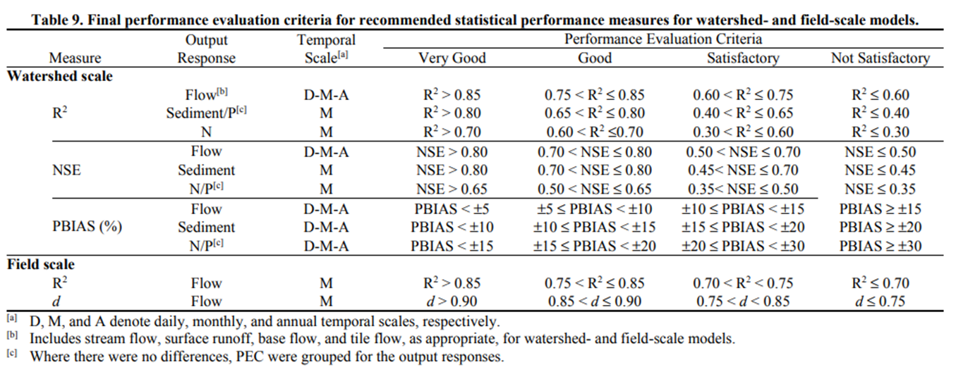
In a spreadsheet, document, or text file, record summary information for the calibrated events Feb 1986, Jan 1997, and Jan 2006. Use the metrics in Moriasi et al., 2015 for the Performance Rating.
Feb 1986 calibration summary:Location
NSE
Performance Rating
Simulated Peak (cfs)
Observed Peak (cfs)
CV Dam Inflow
Ukiah Gage
Hopland Gage
Cloverdale Gage
Healdsburg Gage
Guerneville Gage
Location
NSE
Performance Rating
Simulated Peak (cfs)
Observed Peak (cfs)
CV Dam Inflow
-
-
11,364
11,200
Ukiah Gage
-
-
12,368
12,300
Hopland Gage
-
-
32,598
32,900
Cloverdale Gage
-
-
40,987
40,700
Healdsburg Gage
-
-
71,998
71,100
Guerneville Gage
-
-
106,616
102,000
Jan 1997 calibration summary:Location
NSE
Performance Rating
Simulated Peak (cfs)
Observed Peak (cfs)
CV Dam Inflow
Ukiah Gage
Hopland Gage
Cloverdale Gage
Healdsburg Gage
Guerneville Gage
Location
NSE
Performance Rating
Simulated Peak (cfs)
Observed Peak (cfs)
CV Dam Inflow
0.910
Very Good
7,791
8,270
Ukiah Gage
-
-
11,363
-
Hopland Gage
0.874
Very Good
20,508
20,000
Cloverdale Gage
0.602
Good
29,081
29,000
Healdsburg Gage
0.683
Good
62,438
65,663
Guerneville Gage
0.601
Good
90,088
82,100
Jan 2006 calibration summary:
Location
NSE
Performance Rating
Simulated Peak (cfs)
Observed Peak (cfs)
CV Dam Inflow
Ukiah Gage
Hopland Gage
Cloverdale Gage
Healdsburg Gage
Guerneville Gage
Location
NSE
Performance Rating
Simulated Peak (cfs)
Observed Peak (cfs)
CV Dam Inflow
0.925
Very Good
14,638
14,600
Ukiah Gage
0.921
Very Good
22,250
22,600
Hopland Gage
0.895
Very Good
35,902
35,600
Cloverdale Gage
0.832
Very Good
50,517
50,700
Healdsburg Gage
0.901
Very Good
62,062
58,900
Guerneville Gage
0.710
Good
84,061
86,000
Continue to Create a Validation Parameter Set