Last Modified: 2023-12-13 14:20:47.481

Software Version

HEC-HMS version 4.11-beta.10 was used to create this example. You can open the example project with HEC-HMS v4.11 or a newer version.

Project Files

Download the initial project files here:

SwampAngel_RTI_ParamSens_Start.zip

Introduction

The Gridded Hybrid Snow, or Radiation-derived Temperature Index (RTI), snowmelt method was introduced to HEC-HMS in version 4.11. Information on the Gridded Hybrid Snow method can be found in the HEC-HMS User's Manual and the HEC-HMS Technical Reference Manual. 

The Gridded Hybrid Snow (or Radiation-derived Temperature Index, RTI) method is inherently a gridded method. There is no banded implementation of this snow accumulation and melt model. A terrain and discretization file were developed for you to use the Gridded Hybrid Snow method at a gage, or point, location. 

The following parameters are required to use this method:

• Rain Threshold Air Temperature
• Snow Threshold Air Temperature
• Base Temperature
• Melt Factor
• Max Neg Melt Factor
• ATI Coefficient
• Wind Function
• Water Capacity

In this tutorial, a parameter sensitivity analysis will be performed using the Uncertainty Analysis compute option in HEC-HMS and a regression analysis in Microsoft Excel. In evaluating parameter sensitivity, we are trying to answer the following questions:

• Which parameters play the largest role in the outputs of interest?
• Which parameter should be investigated (and uncertainty reduced) in future efforts?

Study Area

The Swamp Angel Study Plot (SASP) is located in the San Juan Mountains in southwestern Colorado, as shown in the following figure. SASP is located at an elevation of 11,060 ft (3,370 m) and is located in a meadow sheltered by the surrounding terrain and subalpine forest. The location of SASP allows for snowpack and precipitation measurements under minimal wind influence. SASP was used in the Earth System Model-Snow Model Intercomparison Project (ESM-SnowMIP). ESM SnowMIP is an international modeling effort that evaluates snow modeling schemes (Krinner et al. 2018). 

For this tutorial, the study plot is treated as a point location. A simple HEC-HMS model with a single subbasin element was developed. The study plot has an area of 0.22 acres (0.0009 square kilometers).

Finish Model Setup

Create a Meteorologic Model

Before performing a parameter sensitivity analysis, a meteorologic model must be created. Boundary conditions that are required to use the Gridded Hybrid Snow method include:

• Shortwave Radiation
• Longwave Radiation
• Precipitation
• Air Temperature
• Atmospheric Pressure
• Relative Humidity

Meteorological data used in this tutorial was obtained from the ESM SnowMIP data repository. 

1. Download the SwampAngel_HMS_Start project and unzip the file.
2. Start HEC-HMS (version 4.11 or newer) and open the SwampAngel project.
3. Expand the Basin Model folder in the Watershed Explorer and select the SwampAngel basin model. Notice that the basin model contains a single subbasin named SASP.
4. Create a Meteorologic Model by selecting Components | Meteorologic Model Manager. Click the New... button. Name the meteorologic model WY2006 and click the Create button.
5. Close the Meteorologic Model Manager window.
6. Expand the Meteorologic Model folder in the Watershed Explorer and select the InSitu meteorologic model.
7. From the Component Editor, select the following:
   
   • Unit System: U.S. Customary
   • Shortwave: Specified Pyranograph
   • Longwave: Specified Pyrgeograph
   • Precipitation: Specified Hyetograph
   • Temperature: Specified Thermograph
   • Pressure: Specified Barograph
   • Dew Point: Specified Humidograph
   • Evapotranspiration: --None--

   • Replace Missing: Set To Default
     
     The Meteorologic Model component editor should appear as in the figure below.
     
     

      

8. Within the Meteorologic Model Component Editor, navigate to the Basins tab. Under the Include Subbasins header, select Yes from the drop-down menu to link the SwampAngel subbasin to the WY2006 meteorologic model.
   

   

   A Basin Model using the Gridded Hybrid snowmelt method can operate with and be linked to a non-gridded Meteorologic Model. However, when using a gridded Basin Model and gridded Meteorologic Model, it is not necessary to link the Basin Model to the Meteorologic Model.

9. Select the Specified Pyranograph from the Watershed Explorer. Under the Gage header, select SWRadiation from the drop-down menu.
10. Repeat the previous step and make the following selections:
    
    • Specified Pyrgeograph: LWRadiation
    • Specified Hyetograph: Precipitation
    • Specified Thermograph: AirTemperature
      • Lapse Method: --None--
    • Specified Barograph: AirPressure
    • Specified Humidograph: Humidity
11. Save the project.

Create and Compute a Simulation Run

1. Create a Simulation Run by selecting Compute | Create Compute | Simulation Run.... Name the run WY2006_RTI and select the Next button. Select the SwampAngel basin model, the WY2006 meteorologic model, and the WY2006 control specifications on the following screens. Select the Finish button.
2. Select the WY2006_RTI simulation from the Compute Selection Box in the Toolbar.
3. Click the Compute button  to run the simulation.
4. Navigate to the Results tab and expand the Simulation Runs folder.
5. Select the WY2006_RTI simulation and expand the SASP subbasin.
6. Hold the keyboard Ctrl button and select the Observed SWE and Snow Water Equivalent output variables, as shown in the figure below.
   
7. Select the Plot button from the Toolbar. The results should appear as in the figure below.
   

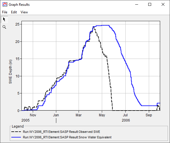
Create and Compute an Uncertainty Analysis

1. Create an Uncertainty Analysis by selecting Compute | Create Compute | Uncertainty Analysis....
2. Name the Uncertainty Analysis U_WY2006_RTI as shown in the figure below. Click the Next> button.
   
3. Select the SwampAngel_RTI basin model. Click the Next> button.
4. Select the WY2006 meteorologic model. Click the Finish button.
5. Navigate to the Compute tab. A few folder titled Uncertainty Analyses was created. Expand the folder and select the U_WY2006_RTI analysis.
6. In the Component Editor, select the gear icon next to the Analysis Points field. Click the checkbox next to the Snow Water Equivalent time series as shown in the figure below.
   
   
7. Click the Save and Close buttons.
8. In the Component Editor, enter the following for the Start Date/Time and End Date/Time:
   
   • Start Date: 02Oct2005
   • Start Time: 0000
   • End Date: 29Sep2006
   • End Time: 0000
9. Select a Time Interval of 1 Hour from the drop-down menu.
10. Enter 1000 in the Total Samples field. The Total Samples refers to the number of times the program will sample new parameter values and run a simulation.
11. Right click on the uncertainty analysis and select Add Parameter.
12. Repeat the above step 7 more times to add a total of 8 parameters.
13. The Rain Threshold Temperature and Snow Threshold Temperature values will be sampled from Specified Values paired data. These sample values are uniformly distributed between -27 deg F and 37.4 deg F. The uniform distribution was used for this parameter sensitivity analysis because no information about parameter distributions was available.
14. In the Watershed Explorer, expand the Paired Data and the Parameter Value Samples folder. Click the RainThresholdTemp node. In the Component Editor, select the Table or Graph tab to view the parameter value samples.
15. Repeat the above step to examine the SnowThresholdTemp values.
16. Return to the U_WY2006_RTI Uncertainty Analysis.
17. Select each parameter node and in the Component Editor, select subbasin SASP in the Element drop-down menu. 

18. For the Rain Threshold Temperature and Snow Threshold Temperature, select Specified Values - Sequential Loop from the Method drop-down menu. Select the appropriate paired data for each parameter. The Parameter tab for Rain Threshold Temperature is shown in the figure below.
    
    

    

    When using the Specified Values - Sequential Loop paired data type, the Uncertainty Analysis will select pair-wise parameters from the tables. In other words, iteration 1 will use the parameter value at index 1, iteration 2 will use the parameter value at index 2, etc.

    When using the Specified Values - Random paired data type, the Uncertainty Analysis will randomly sample from the parameter values in the table. 

    The Specified Values - Sequential Loop paired data type was used to ensure that the Snow Threshold Temperature was less than or equal to the Rain Threshold Temperature for every time step.

19. For the remaining parameters, select Simple Distribution from the Method drop-down menu and Uniform from the Distribution drop-down menu. 

20. Enter the Minimum and Maximum for each parameter using the values in the table below. For the uniform distribution, the Minimum and Lower values are the same and the Maximum and Upper values are the same. Do not enter the units in HEC-HMS; they are provided for clarity. The Parameter tab for Liquid Water Capacity is shown in the figure below.
    
    

    Parameter	Distribution	Minimum	Maximum	Units
    Base Temperature	Uniform	26	37	deg F
    Melt Factor	Uniform	0.003	0.01	in/deg F-6 hr
    Max Neg Melt Factor	Uniform	0.001	0.01	in/deg F-6 hr
    ATI Coefficient	Uniform	0.8	0.99	-
    Wind Function	Uniform	0.5	0.75	in/in Hg-6 hr
    Water Capacity	Uniform	0.1	5	%

    
    
    

21. Turn off notes and warnings in the Message Log by selecting Tools | Program Settings.... Navigate to the Messages tab. Under the Display messages in the message log and Write messages to the log file sections, uncheck the boxes next to Notes and Warnings, as shown in the figure below. Displaying and saving messages increases the run time of the Uncertainty Analysis.
    

22.  Compute the Uncertainty Analysis.
    

    

    The simulation will take approximately 30 minutes to compute. 

Extract Sampled Parameter Values

1. Navigate to the Results tab. Expand the Uncertainty Analyses folder and select the U_WY2006_SwampAngel uncertainty analysis. The Results tab should resemble the figure below. 
   
2. HEC-HMS provides the sampled parameter values for each realization. In addition, the SWE time series and maximum SWE value for each realization are provided. Select a Parameter node to view the sampled parameter values, as in the figure below.
   
   
3. Open each Parameter node and copy the sampled parameter values to an Excel spreadsheet. Include a data label for each parameter (e.g. "Liquid Water Capacity").
4. Expand the SASP subbasin node and select the Maximum SWE time series node. Copy the output to Excel. Include a data label for the maximum SWE output.

Perform a Multiple Linear Regression Analysis in Excel

The parameter values are generated through random sampling. Your parameter values will be different from the values shown in this section unless the same Seed Value is used in the HEC-HMS Uncertainty Analysis. The Seed Value is used to initialize the random number generator. In general, it is not advisable to change the Seed Value unless you are trying to duplicate results. 

1. Compute the mean and standard deviation of each parameter and the maximum SWE using Excel functions AVERAGE and STDEV.S. The Excel spreadsheet should look similar to the figure below. 
   
   
   
2. Before performing a regression analysis, the sampled parameters and maximum SWE output must be standardized. The 8 parameters have different units and scales. Standardization is needed so that parameters with larger standard deviations do not have greater influence on the regression results. In addition, standardization ensures that the regression coefficients have uniform units. The parameters and output were standardized by subtracting the mean and dividing by the standard deviation:
   
   $//<![CDATA[ \begin{array}{l}Z_i = \frac{X_i - \bar{X}}{\hat{\sigma}}\end{array} //]]>$
   
   
3. The mean and standard deviation for each standardized variable should be 0 and 1, respectively. The results of the standardization should look similar to the figure below. 
   
   
   
4. Multiple linear regression can be performed in Excel using the Analysis ToolPak. Select File | Options. Navigate to the Add-ins tab on the left side of the Excel Options dialog box. On the bottom of the dialog box, select Excel Add-ins from the Manage drop-down menu and click the Go... button. Select the check box next to the Analysis Toolpack add-in, as in the figure below. Click the OK button to close the dialog box.
   
   
5. Navigate to the Data tab | Analysis section | Data Analysis option.
6. Select Regression in the Data Analysis dialog box. Click the OK button.
7. In the Regression dialog box, make the following selections:
   
   1. The Input Y Range is the range of cells containing the maximum SWE data (including the data label).
   2. The Input X Range is the range of cells containing the standardized sampled parameters (including the data labels).
   3. Check the Labels box to indicate that data labels were included in the Y and X ranges.
   4. Under the Output Options, enter Results in the field next to New Worksheet Ply to save the regression analysis results in a new tab named Results.
8. The Regression dialog box should resemble the figure below. Click the OK button perform the regression analysis.
   
   
   

Analyze Results

Navigate to the Results tab in Excel. The bottom table (boxed in red in the figure below) shows the results of the regression analysis. The coefficients are used to develop a linear regression of the general form:

$//<![CDATA[ \begin{array}{l}y = ax + b\end{array} //]]>$

where $//<![CDATA[ \begin{array}{l}a\end{array} //]]>$ is the regression coefficient and $//<![CDATA[ \begin{array}{l}b\end{array} //]]>$ is the intercept. In this tutorial, 8 parameters were evaluated. Therefore, the linear regression takes the following form:

$//<![CDATA[ \begin{array}{l}y = a_1x_1 + a_2x_2 + a_3x_3 + a_4x_4 + a_5x_5 + a_6x_6 + a_7x_7 + a_8x_8 + b\end{array} //]]>$

A negative regression coefficient means that smaller parameter values increase the maximum SWE and a positive regression coefficient means that larger parameter values increase the maximum SWE. The P-value indicates whether the dependent variable is statistically significant. Low P-values and high coefficient values indicate that the parameter has a significant impact on the dependent variable, or model output. 

1. Select the 8 parameter labels and the corresponding regression coefficients.

2. Navigate to the Insert tab and select Recommended Charts in the Charts section. Select the Clustered Bar option. Click the OK button. The plot should look similar to the figure below.
   
   
   
   

   

   The results of this parameter sensitivity analysis are specific to the Swamp Angel Study Plot. The regression coefficients for Gridded Hybrid snowmelt parameters will vary by location. A site-specific parameter sensitivity analysis should be performed for your modeling domain.

3. From the tornado chart above, it is easy to tell that the parameters with the greatest impact on the maximum SWE output are the Melt Factor and the Base Temperature. The Base Temperature has the largest positive regression coefficient. The Base Temperature is the temperature above which snow melts. A high Base Temperature increases the temperature range at which snow remains solid, increasing the maximum SWE. The Melt Factor has a negative regression coefficient. A large Melt Factor causes the snow to melt quickly, which reduces the depth of accumulated snow and the maximum SWE. 

4. Another way to evaluate model results is to compare individual model parameters to maximum SWE. Two parameters were selected for further analysis: Wind Function and Base Temperature. The first plot is a comparison between the standardized Wind Function and standardized Maximum SWE. The second plot is a comparison between the standardized Base Temperature and standardized Maximum SWE. The figures show that Base Temperature has a large impact on maximum SWE while Wind Function has very little impact on maximum SWE.  
   
   
   
   
   The results of the regression analysis can inform calibration efforts. In calibrating the Swamp Angel model, the focus should be on parameters related to the melt rate, such as Melt Factor, Base Temperature, and Max Negative Melt Factor. The Excel spreadsheet used to perform the regression analysis is included below.
   

Project Files

Download the final project files here:

SwampAngel_RTI_ParamSens_Finish.zip