Download PDF
Download page Modeling Surface Erosion with Build-up Wash-off Model for Urban Watersheds.
Modeling Surface Erosion with Build-up Wash-off Model for Urban Watersheds
Software
HEC-HMS version 4.13 beta 1 was used to create this example. You can open the example project with HEC-HMS 4.13 or a newer version.
Project Files
Download the Initial Project Files here: BUWO_Initial.zip
Download the HMS Surface Erosion Lecture for useful references: L3.2 HMS Surface Erosion.pptx
Introduction:
This is a continuation from Part 1: Modeling Surface Erosion with MUSLE for Undeveloped Land Areas. For this part of the workshop, a basin model for the urban watershed (U-1, 0.368 mi2) was designed as an impervious segment from theoretical and hypothetical assumptions.
Site description:
Compute the soil loss for U-1 sub-watershed using the Build up and Wash off method in HEC-HMS for the following local conditions:
- Land Use Type: 75% Residential, 5% Commercial, 5 % Industrial, and 15% Park
- # of days after the last storm: 7 days
- The maximum accumulation of solids (Max Solids, LB/MI): 2400 lb/curb mile
- The length of time needed for solid build up to increase from 0 kg/curb km to ½ maximum accumulated solids (Half-Time, DAYS): 7 days
- The fraction of the curb length available for sweeping (Sweeping, %): 80%
- The street cleaning program: 1-pass with Mechanical Street Cleaner (50-500 kg/curb km) per week
- The wash off coefficient (0.039-0.390) (Coefficient, 1/IN): Assume as 0.15
Objectives
Within HEC-HMS, the MUSLE method simulates the sediment yield processes from a pervious land segment and the Build-up and Wash-off method simulates sediment yield processes from an impervious land segment.
The overall goal of the surface erosion workshops is to use the tools in HEC-HMS for sediment erosion calculation from both pervious and impervious land areas. The first objective of this workshop is to determine parameter values and to calculate the sediment loads using MUSLE and Build up and Wash off methods. The second object of this workshop is to calibrate the average annual sediment load using observed data. Explanations are provided to help you estimate reasonable input parameters and to ensure that reasonable sediment loads are calculated. The sediment routing method will be covered in the next workshop.
In this workshop you will simulate surface erosion from impervious land area:
- Develop a surface erosion model in an impervious land segment
- Estimate the sediment loads with designed storm events in an impervious land segment
- Estimate the sediment loads by changing the street cleaning Interval option under similar situations and compare results
- Estimate the sediment loads by changing the Initial Time option under similar situations and compare results
Task 1: Set up the Basin Model for Sediment Transport
- Open the Erosion_Modeling.hms HMS project and click on the Urban WS basin model. In the basin model editor panel, select Yes from the Sediment Transport dropdown to turn on basin sediment transport.
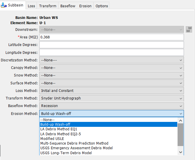
- Select the U-1 subbasin and set the Erosion Method to Build-up Wash-off from the dropdown on the subbasin editor panel. A small window will appear as shown in the figure below. Select Yes to continue. There should now be an Erosion tab on the subbasin editor panel.


Task 2: Estimate Sediment Parameters
Create a gradation curve for your site by selecting Component > Paired Data Manager and selecting Diameter-Percentage Functions as the Data Type. Select New... and name the new paired data component W1. Input the gradation table shown below in the W-1 Table.
| Diameter, MM | Percent Finer, % |
|---|---|
0.0001 | 0.0 |
| 0.0020 | 17.0 |
| 0.0500 | 28.0 |
| 2.0000 | 55.0 |
| 64.0000 | 100.0 |
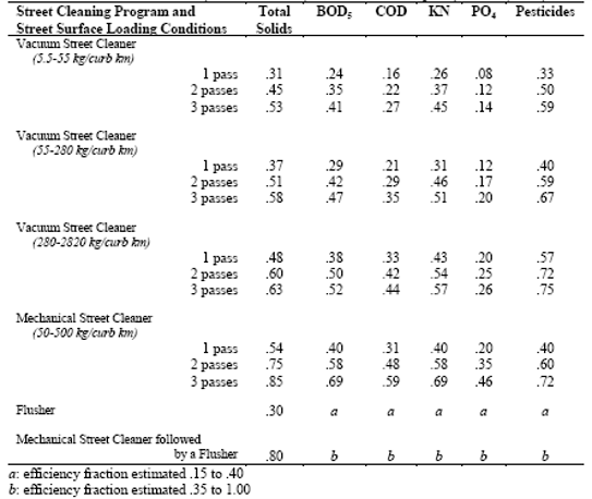
- Reference the information from the site description to determine the erosion parameters. The Interval (DAYS) value represents the interval between sweep operations. The curb length density and sweeping efficiency can be determined based on information on the site description and reference tables shown below.
- Assume the exponent value as 0.75 for the sediment distribution.
- Select the W1 Diameter-Percentage Function from the Gradation Curve dropdown.
Curb Length Density (Heaney et al., 1977; Sullivan et al., 1978)
Land Use | Tulsa, Oklahoma | 10 Ontario Cities | ||||
mi/ac | km/ha | ft/ac | mi/ac | km/ha | ft/ac | |
Residential | 0.076 | 0.300 | 400 | 0.042 | 0.170 | 220 |
Commercial | 0.081 | 0.320 | 430 | 0.057 | 0.230 | 300 |
Industrial | 0.042 | 0.170 | 220 | 0.025 | 0.099 | 130 |
Park | 0.042 | 0.170 | 220 | - | - | - |
Open | 0.016 | 0.063 | 85 | 0.015 | 0.056 | 79 |
Institutional | - | - | - | 0.030 | 0.120 | 160 |
Question 1. Calculate the curb length density using data from Tulsa, Oklahoma (Heaney et al., 1977: Sullivan et al., 1978) based on given information above.
(400 ft/ac × 0.75) + (430 ft/ac× 0.05) + (220 ft/ac × 0.05) + (220 ft/ac × 0.15) = 365.5 ft/ac
Fill in your initial values in the table below.
Parameter | Initial Value |
Initial Time (Days) : | |
Half Build Up Time (Days) | |
Max. Solids Build Up (LB/MI) | |
Curb Length Density (FT/ACRE) | |
Sweeping Percentage of Total Curb Length (%) | |
Removal Efficiency of Sweeping Equipment (%) | |
Interval Between Sweep Operations (Days) | |
Wash Off Coefficient (1/IN) | |
Concentration Distribution Exponent |
Parameter | Initial Value |
Initial Time (Days) : | 0 |
Half Build Up Time (Days) | 7 |
Max. Solids Build Up (LB/MI) | 2400 |
Curb Length Density (FT/ACRE) | 365.5 |
Sweeping Percentage of Total Curb Length (%) | 80 |
Removal Efficiency of Sweeping Equipment (%) | 54 |
Interval Between Sweep Operations (Days) | 7 |
Wash Off Coefficient (1/IN) | 0.15 |
Concentration Distribution Exponent | 0.75 |
Task 3: Compute Simulation Runs and View Results
- Setup a simulation run to compute results. Configure and compute the run with the information below.
- Run name: BUWO
- Basin Model: Urban WS
- Meteorologic Model: U-1-A
- Control Specifications: Jan73
Task 4: Analyze Effect of Street Cleaning
Check the street cleaning effect by changing the operation interval. Fill out the table below.
- Update/Modify the Urban WS basin model with the different operation intervals (Interval (DAYS) given in the table below. Hold all other parameters constant and recompute BUWO simulation. Check the results of Sediment Concentration (Results Tab > Simulation Runs > BUWO> U-1 >Sediment > Sediment Concentration).
- Visually inspect the Sediment Concentration graph and find the concentration magnitudes for each peak in mg/L. Hover the mouse pointer over the peak to see the value displayed.
- Fill in your results in the table below for each of the equipment operation intervals.
Equipment Operation | First Peak | Second Peak |
1-day | ||
3-day | ||
5-day | ||
7-day | ||
9-day | ||
11-day |
Equipment Operation | First Peak | Second Peak |
1-day | 48 | 48 |
3-day | 90 | 75 |
5-day | 108 | 90 |
7-day | 85 | 110 |
9-day | 140 | 156 |
11-day | 140 | 145 |
Question 2: What is the reason that the peak value for the 5-day interval is bigger than the peak value for the 7-day interval?
After the 1st street cleaning, the 5-day interval has 2.5-day for the build up period but the 7-day interval has just 0.5-day for the build up period.
Question 3: What is the reason that the peak value for the 9-day interval is almost same with the peak value for the 11-day interval?
The street cleaning did not happen for these cases because the dry period (7-day) was not longer than the street cleaning intervals (9-day and 11-day).
Task 5: Effect of Initial Time
- Modify the Urban WS basin model with different initial time values given in table below and the fixed 11-day street cleaning interval.
- Check results of Sediment Concentration (Results Tab -> Simulation Runs -> BUWO -> U-1->Sediment -> Sediment Concentration). Fill out the table below with the peak sediment concentrations for the two peaks.
Initial Time | First Peak | Second Peak |
0-day | ||
3-day | ||
5-day | ||
7-day | ||
9-day |
Initial Time | First Peak | Second Peak |
0-day | 140 | 145 |
3-day | 163 | 165 |
5-day | 115 | 175 |
7-day | 136 | 110 |
9-day | 154 | 133 |
Question 4: What is the reason that the first peaks value increased faster than the second peak values?
The first peak is more effected by the initial time because the first peak value is generated based on the initial time and dry period and the second peak value is generated based on the residual value of the first wash off and dry period.
Project Files
