Download PDF
Download page Modeling Surface Erosion with MUSLE for Undeveloped Land Areas.
Modeling Surface Erosion with MUSLE for Undeveloped Land Areas
Software Version
HEC-HMS version 4.13 beta 1 was used to create this example. You can open the example project with HEC-HMS 4.13 or a newer version. HEC-DSSVUE is also required for this tutorial and can be downloaded here: HEC-DSSVue Downloads (army.mil).
Project Files
Download the Initial Project Files here: MUSLE_Initial.zip
Download the HMS Surface Erosion Lecture for useful references: L3.2 HMS Surface Erosion.pptx
Introduction
Hydrological and soil loss data have been collected since 1937 at the USDA-ARS Glassland Soil and Water Research Laboratory near Riesel, TX. Data from the site, originally named the Blacklands Experimental Watershed, have played a vital role in the evaluation of conservation management practices to limit soil erosion and offsite herbicide transport and in the development of several watershed models used worldwide. The entire record of precipitation, runoff, sediment loss, management practices, and limited meteorological information is publicly available (http://www.ars.usda.gov/spa/hydro-data). For the Erosion Modeling Workshop, a W-1 sub-watershed (0.275 mi2 (176 acres)) of the Blacklands experiment watershed was selected as a pervious land segment.
Site Description
The site has highly expansive clays, which shrink and swell with changes in moisture content, have a typical particle size distribution of 17% sand, 28% silt, and 55% clay. This soil series consists of very deep, moderately well-drained soils formed from weekly consolidated calcareous clays and marls and generally occurs on 1-3% slopes in upland areas. This soil is very slowly permeable when wet (approximate saturated hydraulic conductivity of 1.5 mm/hr) (Arnold at al., 2005; Allen et al., 2005). Compute the average annual soil loss for W-1 sub-watershed using MUSLE model in HEC-HMS for the following conditions: cropland, contour strip-cropped slopes are 2.2%, and 260-ft (79.25-m) long. W-1 sub-watershed is a mixed landuse area so C and P values are assumed (C=0.95 and P=0.18).

Objectives
Within HEC-HMS, the MUSLE method simulates the sediment yield processes from a pervious land segment and the Build up and Wash off method simulates sediment yield processes from an impervious land segment.
The overall goal of the surface erosion workshops is to use the tools in HEC-HMS for sediment erosion calculation from both pervious and impervious land areas. The first objective of this workshop is to determine parameter values and to calculate the sediment loads using MUSLE and Build up and Wash off methods. The second object of this workshop is to calibrate the average annual sediment load using observed data. Explanations are provided to help you estimate reasonable input parameters and to ensure that reasonable sediment loads are calculated. The sediment routing method will be covered in the next workshop.
In this workshop you will simulate surface erosion from pervious land area:
- Develop a surface erosion model in a pervious land segment
- Estimate the sediment loads with the calibrated watershed model
- Calibrate the model in terms of an average annual sediment load with 10-year (01Jan1961-31Dec1970) of sediment load data
- Validate the model in terms of an average annual sediment load with 10-year (01Jan1971-31Dec1980) of sediment load data
Task 1: Set up the Basin Model for Sediment Transport
- Open the Erosion_Modeling.hms HMS project and click on the Riesel W-1 basin model. In the Basin Model Editor Panel, select Yes from the Sediment Transport dropdown to turn on basin sediment transport.
- Select the W-1 subbasin and set the Erosion Method to Modified USLE from the dropdown on the subbasin editor panel. A small window will appear as shown in the figure below. Select Yes to continue. There should now be an Erosion tab on the subbasin editor panel.


Task 2: Estimate Sediment Parameters
Create a gradation curve for your site by selecting Component > Paired Data Manager and selecting Diameter-Percentage Functions as the Data Type. Select New... and name the new paired data component W1. Input the gradation table shown below in the W-1 Table.
| Diameter, MM | Percent Finer, % |
|---|---|
0.0001 | 0.0 |
| 0.0020 | 17.0 |
| 0.0500 | 28.0 |
| 2.0000 | 55.0 |
| 64.0000 | 100.0 |
- Determine the soil texture using the Soil Texture Calculator | Natural Resources Conservation Service (usda.gov) input the particle size percentages for clay, sand and silt to determine the predominant soil class.
- Reference the information from the site description and references below to determine the soil erodibility factor (K), topographic factor (LS), cover factor (C), and practice factor (P).
- Assume the exponent value as 0.75 for the sediment distribution.
- Use a flow threshold of 5 cfs and save the basin model.
 NOTE: Do NOT use the default flow threshold of 0.0 cfs. This will lead to the model interpreting the whole time series as a single event.
 - Select the W1 Diameter-Percentage Function from the Gradation Curve dropdown.

The erodibility factor can be estimated from the Wischmeier and Smith Table (1965) and the topographic factor can be estimated from the USDA-SCS Graph. Both are shown below.
")

Estimates of Erodibility Factor, K, by source | ||||
Wischmeier and Smith Table (1965) | Wischmeier at al. EQ (1971)* | William EQ (1995) | SSURGO | USDA-ASR Local |
0.29 | 0.17 | 0.15 | 0.32 | 0.27 |
| Estimates of Erodibility Factor, LS, by source | ||
EQ | USDA-SCS Graph | USDA-ASR Local |
0.30 | ~0.27 | 0.29 |
| Final Initial Parameter Estimates | |||||
K | LS | C | P | Threshold | Exponent |
0.29 | 0.27 | 0.95 | 0.18 | 5.0 | 0.75 |
Task 3: Run Simulation and View Results
- Setup a simulation run to compare results. Configure and compute the run with the information below:
- Run name: MUSLE
- Basin Model: Riesel-W-1
- Meteorologic Model: W-2-A
- Control Specifications: 10-yr Calibration
- Use HEC-DSSVue to open the output DSS file MUSLE.dss
- Select the pathname: //W-1/SEDIMENT LOAD/01JAN1961 – 01DEC1975/15MIN/RUN:MUSLE/.
Calculate the total sediment load with the DSS Utilities. Tools > Math Functions. Select the Statistics Tab and then use the Accumulated Amount for the total sediment load. Answer the questions below.

Question 1: What is the total accumulated sediment load?
4231 TONS
Question 2: What is the annual average sediment load calculated?
4231 TONS / 10 YEARS = 423 tons/year
The average annual sediment load between 01JAN1961 and 31DEC1970 from the field measured data is 14.68 tons/acre. This data was found at the Riesel Daily Sediment Records : USDA ARS website.
Question 4: What is the difference between the computed and observed averaged annual sediment load?
The subbasin area is 0.275 square miles: 0.275 sq. mi x 640 acre/sq mi = 176 acres. 14.68 tons/acre x 176 acres / 10 years = 258 tons/year
423 tons/year - 258 tons/year = 165 tons/year
Task 7: Model Calibration
At this point, you are ready to put together your best model, and make any final parameter adjustments using observed sediment yield data. The idea here is to calibrate your model so that it produces results that compare well to the observed data by making some adjustments if there are any discrepancies.
- Using the Riesel-W-1 basin model, enter your revised C, K, P, LS and Threshold values in the Modified USLE Erosion component editor.
- Run your model using the previously created run, MUSLE, consisting of the Riesel-W-1 basin model, the W-2-A meteorologic model and the 10-yr Calibration control specifications.
- Calibrate your model manually using observed average annual sediment load. Decide on parameter changes that will help improve the fit between computed and observed average annual sediment load. Repeat this process several times in an attempt to match the simulated and observed values. There are some guiding principles below that might help you.
- Fill in your final values in the table below.
Parameter | Initial Value | Calibrated Value |
Cover Factor (C) | 0.95 | |
Erodibility Factor (K) | 0.29 | |
Practice Factor (P) | 0.18 | |
Topographic Factor (LS) | 0.27 | |
Event Flow Threshold | 5.0 | |
Average Annual Sediment Load (ton/yr) | 423 |
Parameter | Initial Value | Calibrated Value |
Cover Factor (C) | 0.95 | 0.95 |
Erodibility Factor (K) | 0.29 | 0.29 |
Practice Factor (P) | 0.18 | 0.18 |
Topographic Factor (LS) | 0.27 | 0.27 |
Event Flow Threshold | 5.0 | 30 |
Average Annual Sediment Load (ton/yr) | 423 | 313 |
Task 8: Model Validation
At this point, you are ready to validate your best model using an additional 10-year of observed sediment yield data (01JAN1971 – 31DEC1980). The idea here is to verify that your model also produces results that compare well to the observed data extended.
- Using the Riesel-W-1 basin model, make sure the calibrated C, K, P, LS and Threshold values have been entered into the Modified USLE Erosion component editor.
- Setup a simulation run to validate results. Configure and compute the run with the information below:
- Run name: MUSLE-Validation
- Basin Model: Riesel-W-1
- Meteorologic Model: W-2-A
- Control Specifications: 10-yr Validation
3. Run your model using the MUSLE-Validation.
The average annual sediment load between 01JAN1971 and 31DEC1980 from the field measured data is 4.21 tons/acre. This data was found at the Riesel Daily Sediment Records : USDA ARS website.
Question 5: What was the average annual sediment load for the validation simulation period?
5501 TONS / 10 YEARS = 550 tons/year
Task 9: Create Uncertainty Analysis - Surface Erosion Parameters
Uncertainty for surface erosion parameters using the Uniform Distribution and example values.
Parameter | Min/Lower | Max/Upper |
|---|---|---|
Erodibility Factor | 0.03 | 0.69 |
Topographic Factor | 0.1 | 1.0 |
Cover Factor | 0.85 | 0.97 |
Practice Factor | 0.1 | 0.3 |
- Set up an uncertainty analysis for surface erosion parameters for the Jan73 event using the Riesel-W-1 basin model and the W-2-A meteorological model. This is done by opening Compute | Uncertainty Analysis Manager.
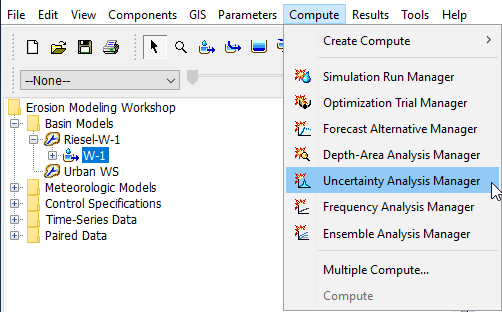 Uncertainty Analysis Manager
- Create a New Uncertainty Analysis and name it MUSLE_Factor.
- Select the MUSLE_Factor Uncertainty Analysis compute and navigate to its Component Editor. Analysis Points controls the computed outputs that are saved and viewable as results. It defaults to Selected since the user is required to choose which outputs to save. Select the cog wheel
 by the Analysis Point to choose your outputs.
- Under Include Analysis Point, check Sediment Load at W-1 so you only need to add parameters for the W-1 sub-basin. Select Save then Close. This is seen in the figure below.
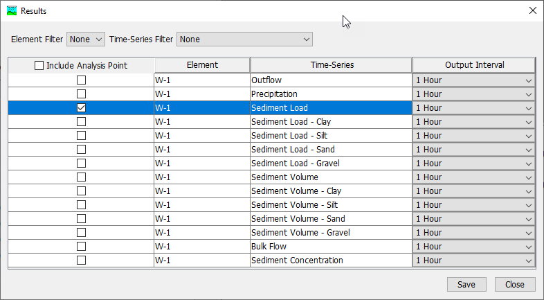 Selecting Analysis Points Output Results
 - Set the time window for Jan73 (08Jan1973 16:00 to 26Jan1973 13:00).
Choose 50 Total Samples (in the interest of time, this should take about 1 minutes to compute) and use the default Seed Value.
Your default seed value will be different than the seed value used in the demonstration and therefore your results will look different. The seed value initializes the pseudorandom number generator that creates the parameter random samples. The same seed will always produce the same random numbers, so two uncertainty computes with the same settings and seed will always produce the same results. The seed value is initialized by the system clock when a new uncertainty compute is created.
- Add a sensitivity parameter to the Uncertainty Analysis using the Simple Distribution sampling for Constant Loss Rate.
- Right click on MUSLE_Factor and select Add Parameter
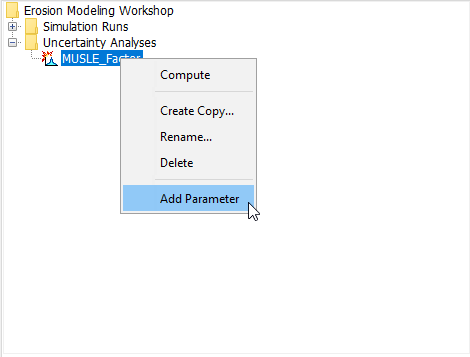 Adding a Parameter for Uncertainty Analysis
 - Select Parameter 1 and in its Component Editor, choose W-1 as the Element
- Select Modified USLE - Soil Erodibility Factor for Parameter, select Simple Distribution for Method, select Uniform for Distribution
- Use the Table above to input the Lower and Upper and Minimum and Maximum values. The Lower and Upper are used to populate the Uniform Distribution parameters, a and b. The Minimum and Maximum are value limits that are imposed after the random sampling (i.e. if the random sample is within the min and max limits, the sample is kept and used for the analysis).
- Right click on MUSLE_Factor and select Add Parameter
- Add parameters for the W-1 subbasin Modified USLE - Topographic Factor, Modified USLE - Cover Factor, and Modified USLE - Practice Factor. Make sure your parameter ranges won’t cause errors, such as a Max Deficit value less than the Initial Deficit already in the basin model. Example values are provided for you in the Table above. You should have a total of 4 Parameters
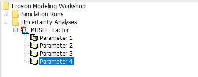 Four Surface Parameters
 - Run your uncertainty analysis for the surface parameters.
- After completing the run (50 iterations should take about 1 minutes or less) open the results in HEC-HMS by selecting the Results tab
- Select Parameter 1 to view the sampled constant loss rate. You should see a total of 50 values.
- Select W-1 to view Sediment Load, Sediment Load Total Maximum, and Sediment Load Total. Sediment Load displays summary statistics of the 50 computes - Mean, Maximum, Minimum, Mean Plus 1 Std Dev, and Mean Minus Std Dev. The summary graphs are computed by taking all of the 50 simulation flow timeseries and computing the metric value for every timestep.
Question 6: How would you determine which sampled parameter set computed the largest sediment load value? Where can you go to see the outflow hydrograph?
Review the Sediment Load Total Maximum table in the Results tab and find the largest peak sediment load value. The Sample Number to the left of the value indicates the sample position.
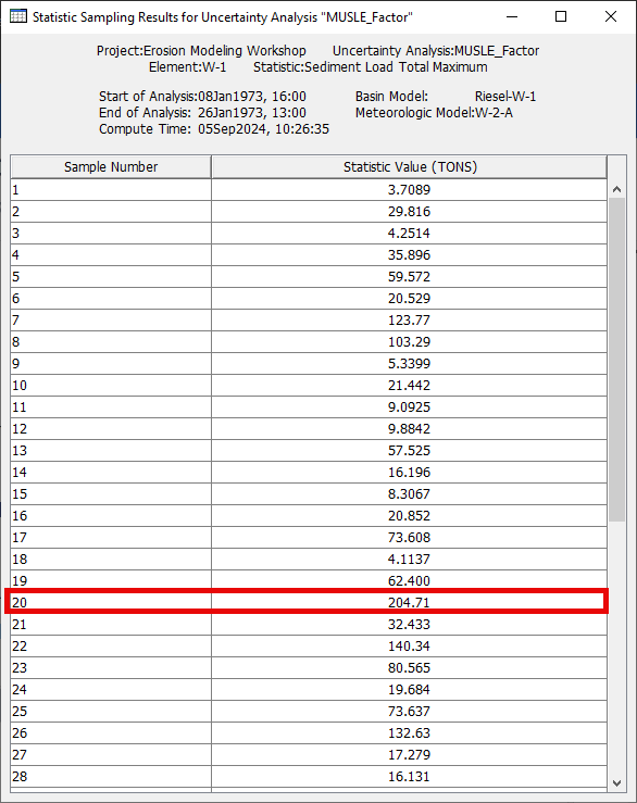
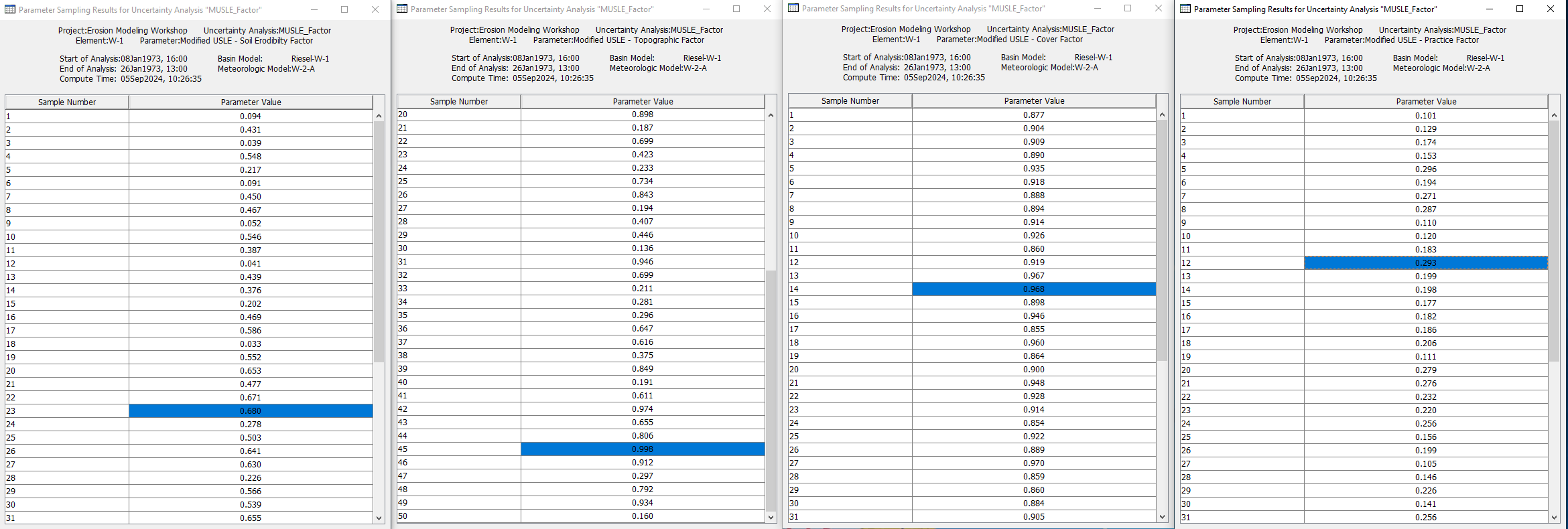
Heading over to the Parameter tables, look for the position number to find the parameters that computed the largest peak value.
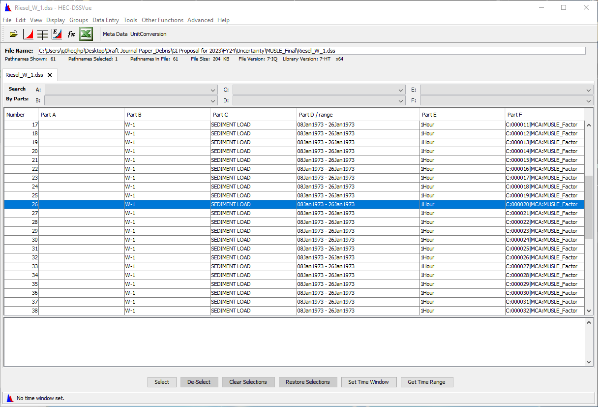
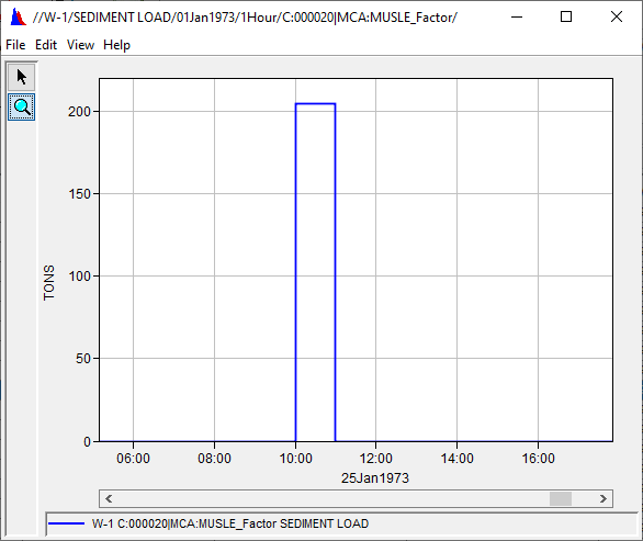
To view the timeseries output, head over to the project folder and open the Riesel_W_1.dss file. In the Part F, look for the position number. This record contains the timeseries sedigraph that computed the highest peak sediment load.
Project Files
Download the Final Project Files here: MUSLE_Final.7z
Continue on to Modeling Surface Erosion with Build-up Wash-off Model for Urban Watersheds.