Review the Existing HEC-HMS Project

HEC-HMS version 4.12-beta.5 was used to create this tutorial.  You will need to use HEC-HMS version 4.12, or newer, to open the project files.

Download the initial model files here:

PMF_Workshop_B_Initial.zip

Simulate Historical Events

1. Launch HEC-HMS and open the PMF_Workshop_B project.
2. Select the Basin Models folder to expand the Watershed Explorer and see all basin models in this project.
   1. You should notice a separate basin model for each historical event (1972, 1996, and 2004).
   2. The fourth Basin Model, named PMF_UH_peak25, was created as a place holder for the final set of model parameters to be used in the PMF simulation.
3. Run all three of the historical simulations.
   
   

   You can run multiple simulations by selecting Compute | Multiple Compute, clicking Select All, and clicking Compute.

4. Compare model output at the Computation Points.
   
   

   You can access the model output by expanding the simulation runs under the Results tab. All computation points are highlighted with a red box around the element icon.

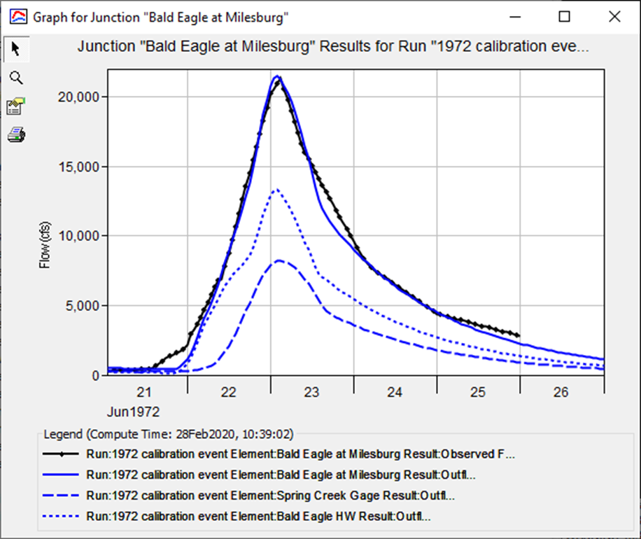
   1. The figure below shows the computed and observed flood hydrographs at the Bald Eagle at Milesburg junction for the 1972 event.
      
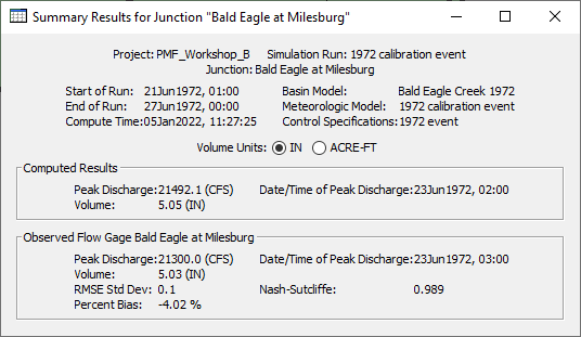
   2. You should notice the model does a good job reproducing the observed flow for these three events.  The reported Nash-Sutcliffe Efficiency (NSE) shows good model performance, as shown in the following image.
      

Note Calibrated Model Parameters

Losses

According to ER 1110-8-2, loss parameters used when simulating the PMF event should “be derived to correspond to patterns favorable for rapid concentrations of runoff from the drainage basin”.  Typically, the lowest loss rates used during model calibration would be used for the PMF simulation, unless loss rates were unreasonable due to poor quality precipitation or flow observations.  ER 1110-8-2 also states that loss parameters need to be adjusted to account for wet antecedent conditions in the watershed at the beginning of the PMF simulation (assumption of a rainfall-runoff event occurring before PMF event).

Question 1: Based on the description above, what do you think is an appropriate Constant Loss Rate parameter to use when simulating the PMF?  Keep track of your parameter values in a spreadsheet.

The initial loss should be set to a reasonable value that reflects an antecedent storm occurring 3-5 days prior to the PMF.  Evapotranspiration will remove some surface and soil water, and water in the soil will percolate so that field capacity is reached.  The time of the year should be considered as well since the moisture deficit grows more quickly in warmer months.  For this workshop, an Initial Loss of 0.5 inches will be used because the PMF will likely occur between spring and fall months.

Unit Hydrograph Transform

Later steps will focus on adjustments to the unit hydrograph and reach routing parameters.  For now, note the Time of Concentration (Tc) and Storage Coefficient (R) parameters in a spreadsheet for all three calibration events as well as the average.

The Tc and R for each subbasin can be seen by accessing the Global Editor Parameters | Transform | Clark Unit Hydrograph.

Question 2: What were the calibrated Tc and R for each historical event?  Compute the average Tc and R for each subbasin as well.

Reach Routing

Note the calibrated Muskingum parameters for the Bald Eagle 40 routing reach in a spreadsheet.

Question 3: What were the calibrated Muskingum parameters for each historical event?

Baseflow

Note the calibrated baseflow parameters in a spreadsheet.

It is important to verify that baseflow parameters do not result in unrealistic runoff volumes for the PMF simulation.  Precipitation and runoff volumes should be compared to ensure that mass is conserved (i.e., precipitation > runoff).  For most studies, the Ratio-to-Peak parameter used when calibrating the model to historic floods will not be appropriate for the PMF simulation.  The Ratio-to-Peak parameter controls when the baseflow recession curve begins on the falling limb of the runoff hydrograph.

Question 4: What were the calibrated Recession baseflow parameters for each historical event?

Continue to Simulating the PMF Using the Clark Method.