Download PDF
Download page Applying the Uncertainty Analysis Compute Option in HEC-HMS.
Applying the Uncertainty Analysis Compute Option in HEC-HMS
Last Modified: 2024-06-11 12:35:30.719
Software Version
HEC-HMS version 4.13-alpha was used to create this tutorial. You can open the example project with HEC-HMS v4.13 or a newer version.
Background
Hydrologic models are subject to various types of uncertainty that can affect the accuracy of their predictions. The sources of uncertainty can be classified into four types: model parameter, model structure, observations, and input data. Understanding, accounting for, and communicating uncertainties associated with hydrologic modeling predictions can help modelers and decision makers make better informed decisions.
A few situations where exploring the model parameter sensitivity could be useful to a modeler:
- Prior to model calibration or model forecasting and deciding which parameters to change
- After stochastic optimization to see the impact of the plausible parameter sets on the results
- During model validation, using the uncertainty caused by differing parameters across calibration events in expressing uncertainty in validation
- When estimating the magnitude of a design event such as the probable maximum flood (PMF) which is subject to tremendous uncertainty
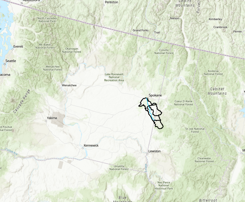
In this workshop, parameter uncertainty will be explored. Parameter uncertainty arises from the fact that values of model parameters, such as soil infiltration, are not known precisely. HMS contains several methods for varying a model’s parameters based on random sampling, and in this workshop you will explore the Simple Distribution sampling method. You will evaluate the sensitivity of the Latah Creek watershed’s outflows to variation in runoff parameters. Latah Creek watershed is located in eastern Washington and north central Idaho. The Latah Creek (also known as Hangman Creek) originates from the Rocky Mountains and flows northwest towards the city of Spokane before it merges with the Spokane River (some interesting history and geology of the area: http://www.sevenwondersofwashingtonstate.com/the-channeled-scablands.html).
Goal
This watershed has significant runoff contribution caused by snowmelt, but it is uncertain whether the rate of melt and the intensity of rainfall makes the surface runoff processes (i.e. infiltration and transform) more sensitive, or if the interflow/baseflow processes are dominant.
This workshop provides example distributions and parameter values for the user to test; however, these distributions and values are for demonstration purposes only. Users are encouraged to try different distributions and parameter ranges.
User's Manual
For more detail on the available distributions in HEC-HMS, see the User's Manual section here: Uncertainty Analyses - Monthly Distribution.
An HEC-HMS model of the Latah Creek watershed is provided above as well as an excel spreadsheet to input your computed parameter results.
Create Uncertainty Analysis - Surface Parameters
Uncertainty for surface parameters using the Uniform Distribution and example values.
Parameter | Min/Lower | Max/Upper |
|---|---|---|
Constant Rate | 0.0 | 1.0 |
Storage Coefficient | 1.0 | 24.0 |
Time of Concentration | 1.0 | 24.0 |
Maximum Deficit | 6.0 | 18.0 |
- Set up an uncertainty analysis for surface parameters for the 2017 event using the Latah Creek basin model and the DerivedGauges2017 meteorological model. This is done by opening Compute | Uncertainty Analysis Manager.
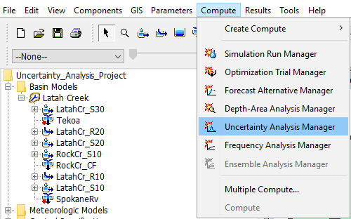
- Create a New Uncertainty Analysis and name it Tekoa_Surface.
- Select the Tekoa_Surface Uncertainty Analysis compute and navigate to its Component Editor. Analysis Points controls the computed outputs that are saved and viewable as results. It defaults to Selected since the user is required to choose which outputs to save. Select the cog wheel
 by the Analysis Point to choose your outputs.
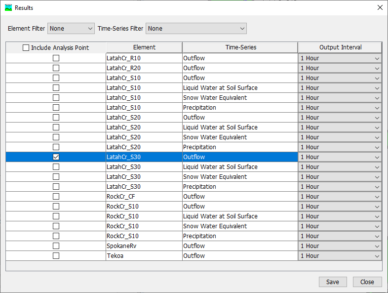
- Under Include Analysis Point, check Outflow at LatahCr_S30 so you only need to add parameters for the LatahCr_S30 sub-basin. Select Save then Close. This is seen in the figure below.
- Set the time window for water year 2017 (01Oct2016 00:00 to 30Sep2017 00:00).
Choose 50 Total Samples (in the interest of time, this should take about 5 minutes to compute) and use the default Seed Value.
Your default seed value will be different than the seed value used in the demonstration and therefore your results will look different. The seed value initializes the pseudorandom number generator that creates the parameter random samples. The same seed will always produce the same random numbers, so two uncertainty computes with the same settings and seed will always produce the same results. The seed value is initialized by the system clock when a new uncertainty compute is created.
- Add a sensitivity parameter to the Uncertainty Analysis using the Simple Distribution sampling for Constant Loss Rate.
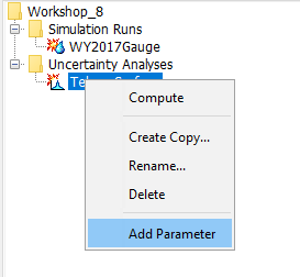
- Right click on Tekoa_Surface and select Add Parameter
- Select Parameter 1 and in its Component Editor, choose LatahCr_S30 as the Element
- Select Deficit and Constant - Constant Loss Rate for Parameter, select Simple Distribution for Method, select Uniform for Distribution
- Use the Table above to input the Lower and Upper and Minimum and Maximum values. The Lower and Upper are used to populate the Uniform Distribution parameters, a and b. The Minimum and Maximum are value limits that are imposed after the random sampling (i.e. if the random sample is within the min and max limits, the sample is kept and used for the analysis).
- Right click on Tekoa_Surface and select Add Parameter
- Add parameters for the LatahCr_S30 subbasin Clark Unit Hydrograph - Storage Coefficient, Clark Unit Hydrograph - Time of Concentration, and Deficit and Constant Max Deficit. Make sure your parameter ranges won’t cause errors, such as a Max Deficit value less than the Initial Deficit already in the basin model. Example values are provided for you in the Table above. You should have a total of 4 Parameters
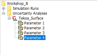
- Run your uncertainty analysis for the surface parameters.
- After completing the run (50 iterations should take about 5 minutes or less) open the “xlsx” spreadsheet and start with the “Max Outflow – Surf” worksheet.
- Open the results in HEC-HMS by selecting the Results tab
- Select Parameter 1 to view the sampled constant loss rate. You should see a total of 50 values.
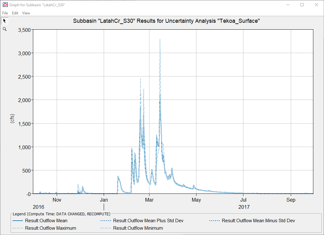
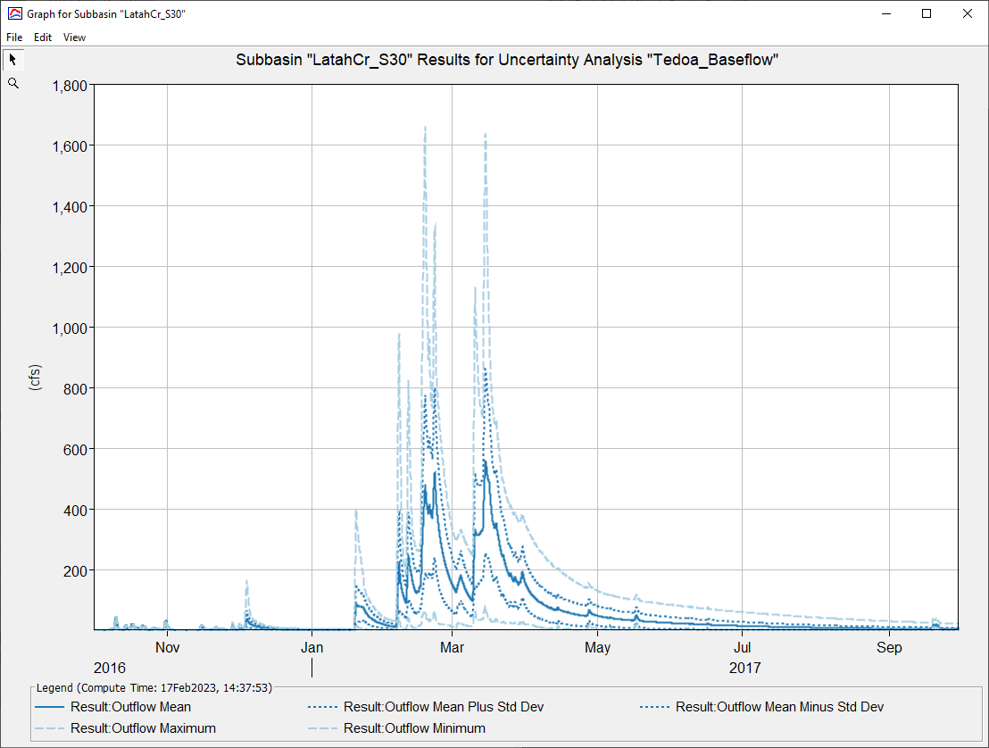
- Select LatahCr_S30 to view Outflow, Maximum Outflow, and Outflow Volume. Outflow displays summary statistics of the 50 computes - Mean, Maximum, Minimum, Mean Plus 1 Std Dev, and Mean Minus Std Dev. The summary graphs are computed by taking all of the 50 simulation flow timeseries and computing the metric value for every timestep.
- Once you finish looking over the results, open the Maximum Outflow table and paste in the max outflow results in column C in the spreadsheet.
- Add in the parameter values (Parameters 1 - 4) in columns D through G. The plots on the right side will update.
- Repeat this procedure on the “Volume – Surf” tab worksheet with the Outflow Volume table. The parameter values should update but you will need to paste in the volumes. If values do not update, paste in the parameter values into each column.
- Review the generated spreadsheet plots. In some cases, you may need to zoom in on the y-axis where the majority of the points are to better analyze trends.
You can zoom in on the y-axis by right-clicking on the y-axis, selecting Format axis..., and then changing the minimum and maximum bounds.
- Open the results in HEC-HMS by selecting the Results tab
Question: Which surface parameter do you think was most sensitive for peak discharge and for the volume of discharge? Are these simulations conclusive?
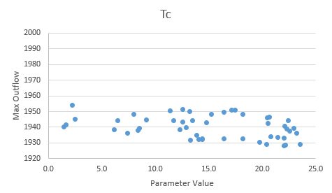
Plots may differ from person to person. The plots seem to indicate none of these parameters are particularly sensitive to the peak outflow. One instance of a lowest constant rate resulted in the highest peak value.
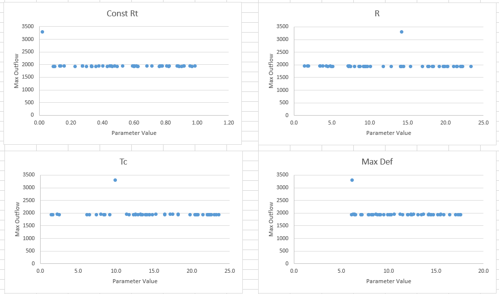
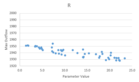
By zooming into the Storage Coefficient and Time of Concentration, the plots indicate a slight negative trend (increasing R or Tc decreases peak value) though it doesn't appear the parameters are sensitive to changes.
For volumes, two instances of a low max deficit resulted in higher volumes.
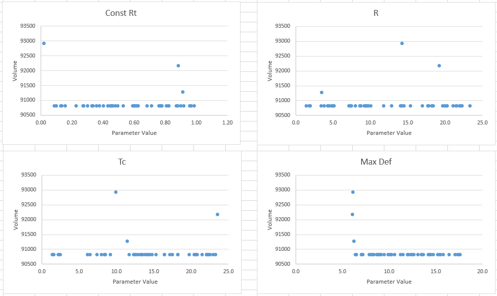
The simulations here are inconclusive. Consider running more simulations.
Question: How would you determine which sampled parameter set computed the largest peak flow value? Where can you go to see the outflow hydrograph?
Review the Maximum Outflow table in the Results tab and find the largest peak flow value. The Sample Number to the left of the value indicates the sample position.
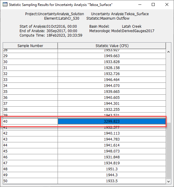
Heading over to the Parameter tables, look for the position number to find the parameters that computed the largest peak value.
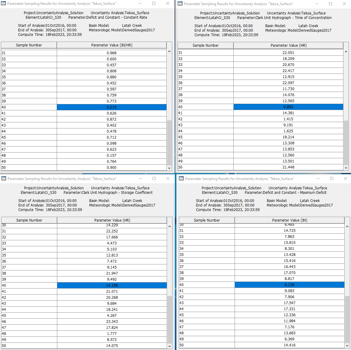
To view the timeseries output, head over to the project folder and open the Tekoa_Surface.dss file. In the Part F, look for the position number. This record contains the timeseries hydrograph that computed the highest peak outflow.
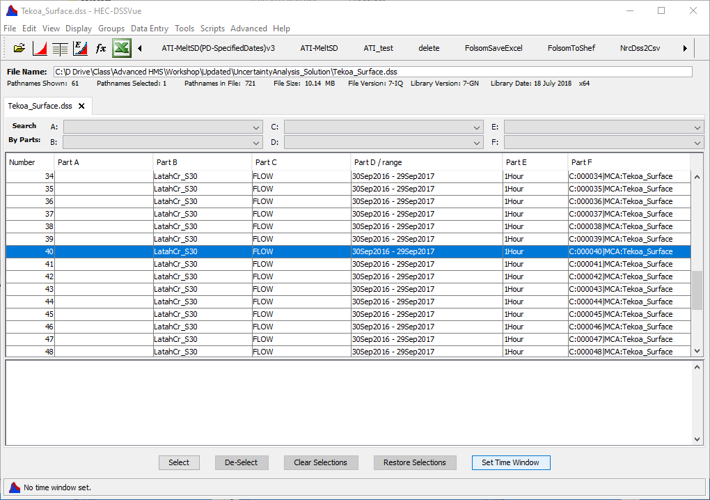
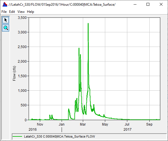
Question: How does your choice setting the uncertainty distribution for a parameter affect the range of outputs?
If unreasonably large or small values are sampled, potentially unreasonably large or small outputs might result. For sensitive parameters, a wide range of input will result in a big spread in the output. In the example above, a few samples for the constant loss rate parameter were close to a value of zero and resulted in large peak flows. These low constant loss rates may not be reasonable for this watershed and the user may consider adjusting the parameter range.
Question: Based on your results, do you think 50 simulations is enough to really evaluate the range of parameter combinations? Why or why not?
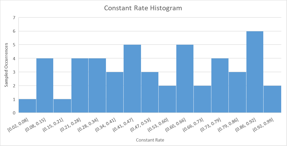
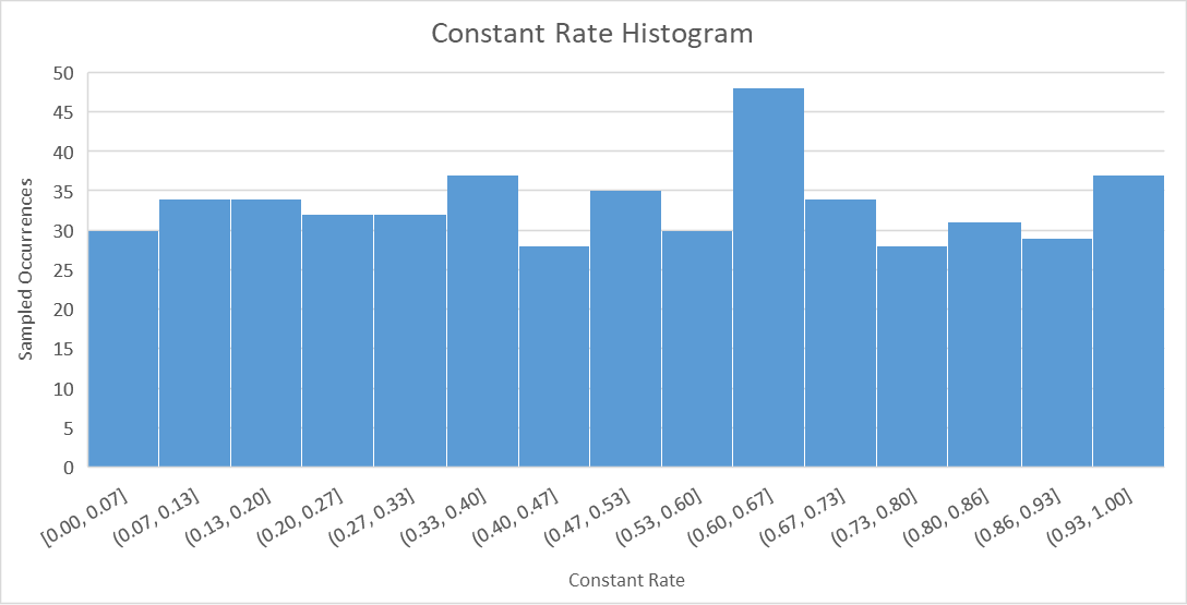
50 is a very small sample size and it’s unlikely that all of the combinations of four parameters in various ranges has occurred; some of the signal might be lost. The parameters are sampled from a uniform distribution. With enough samples, a histogram plot of the sampled parameters should begin looking like the uniform distribution. For example, the first histogram below represents the frequency that constant rate values (within a specific range) were sampled using a sample size of 50 and a uniform distribution. The second histogram represents a sample size of 500. The second histogram more accurately resembles a uniform distribution.
Create Uncertainty Analysis - Baseflow Parameters
Uncertainty for baseflow parameters using the Triangular Distribution and example values
Parameter | Min/Lower | Mode | Max/Upper |
|---|---|---|---|
GW 1 Coeff | 1.0 | 150 | 240.0 |
GW 2 Coeff | 240.0 | 1500 | 2400.0 |
Uncertainty for baseflow parameters using the Exponential Distribution and example values.
Parameter | Shift | Mu | Min | Max |
|---|---|---|---|---|
GW 1 Fraction | 0 | 0.25 | 0 | .5 |
GW 2 Fraction | 0 | 0.25 | 0 | .5 |
- Create a new uncertainty simulation for the baseflow parameters using the same settings. You can also make a copy the existing Tekoa_Surface uncertainty analysis and change the parameter values.
- Create a New Uncertainty Analysis and name it Tekoa_Baseflow.
- Select Tekoa_Baseflow and navigate to its Component Editor. The Analysis Points controls the computed outputs to save and view results. Select the cog wheel
 by the Analysis Point to choose your outputs.
 - Under Include Analysis Point, check Outflow at LatahCr_S30 so you only need to add parameters for the LatahCr_S30 sub-basin. Select Save then Close.
- Right click Tekoa_Baseflow and select Add Parameters
- Add parameters for GW1 Coefficient, GW2 Coefficient, GW1 Fraction and GW2 Fraction. Choose a distribution method and provide its parameters based on the current basin model parameters. Example distributions and their parameters are listed in the table above.
- Record the results in the “Max Outflow – BF” and “Volume – BF” worksheets.
- Review your results for the two analyses. Look at the outflow hydrograph for Tekoa for each of the analysis.
Question: Which baseflow parameter do you think was most sensitive for peak discharge, and for the volume of discharge?
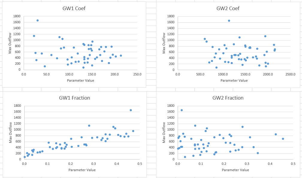
Results may differ from person to person. Though highly variable, the GW 1 coefficient has a signal for peak discharge (negatively correlated) where lower GW 1 coefficient can produce high peak flows. GW 1 Fraction has a clear positive signal (as the fraction increases, the peak outflow increases). The others are more nebulous.
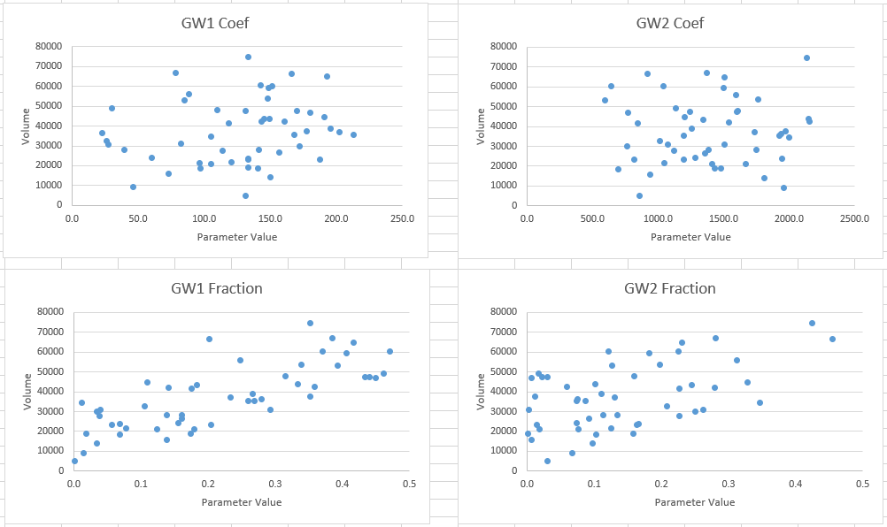
GW 1 & 2 coefficients do not appear to affect volume much. As you would expect, the GW fractions have a very clear signal with volume.
Question: Between surface flow and interflow/baseflow, which do you think has more influence on the runoff process in this sub-basin?
Based on the sensitivity, it seems this is a baseflow/interflow-dominated system. Changes to the baseflow parameters have a large effect on the resulting flows. Without incorporating baseflow, your model will likely miss an important hydrologic process and not calibrate or perform well.
Question: When performing a sensitivity analysis, how is the interaction or dependency between the parameters handled? What is a tool in HMS that can help you analyze that dependency?
These parameters are sampled independently. This means that implausible combinations of parameters might be sampled because sampling is not considering the joint distribution of the parameters. The simple distributions as defined are for the marginal distribution of the parameters. The Linear regression with error method can introduce relationships between parameters.
Create an uncertainty analysis with the regression relationship
Assume, through your investigation and calibration efforts, you determined a linear relationship between GW1 Coefficient and GW2 Coefficient. The linear regression parameters are shown in the table below. The final solutions spreadsheet provided at the end of this tutorial shows how the slope and intercept values were determined.
| Slope | Intercept |
|---|---|
| 7.2051 | 432.62 |
From the regression analysis, you also were able to determine the regression error.
| Distribution | Lower | Mode | Upper |
|---|---|---|---|
| Triangular | -400 | 0 | 400 |
We will use this GW1 and GW2 regression relationship to parameterize the GW 2 Coefficient.
- Copy the existing Tekoa_Baseflow uncertainty analysis and rename the analysis to Tekoa_Baseflow_reg.
- Select Tekoa_Baseflow_reg and navigate to its Component Editor.
- Select Parameter 2 (or whichever one that has Parameter set to Linear Reservoir - GW 2 Coefficient (2)
- Change Method to Regression With Additive Error
- Select LatachCr_S30 for the Reg Element and Linear Reservoir - GW 1 Coefficient (1) as the Reg Parameter
- Set Regression to Linear and Distribution to Triangular. This distribution is describing the uncertainty surrounding the epsilon (error).
- Enter the values from the table above
- Compute the Uncertainty Analysis and record your results in the “Max Outflow – BF_reg” and "Volume - BF_reg" worksheets.
Question: How does the results with the linear regression relationship compare with the baseflow results without the regression relationship?
The GW 2 Coefficient plot looks more similar to the GW 1 Coefficient plot as opposed to the plots before without the regression relationship since the GW 2 coefficient is now directly related to the value selected for GW 1. The max outflow values are not significantly impacted with this inclusion, though including the regression relationship would better reflect the uncertainty surrounding the baseflow hydrograph.

Create Uncertainty Analysis - Snowmelt Parameters
HEC-HMS has the ability to perform uncertainty analyses of many Temperature Index Snowmelt process parameters. It turns out that while the hydrologic process uncertainty is substantial for Latah Creek, the snow model might be just as important. Nearby SNOTEL sites which are higher in elevation (e.g. Moscow Mountain, Sherwin) accumulate 5 – 20 inches of peak SWE in a normal year. Tekoa is down in the valley but plenty of the Latah Creek watershed has enough elevation to create orographic uplift and enhanced precipitation in the watershed, where otherwise it is very dry.
Parameter | Min/Lower | Max/Upper |
|---|---|---|
Px Temperature | 30 | 37 |
Rain Rate Limit | 0 | 0.5 |
Wet Melt Rate | 0.05 | 0.2 |
- Create a third uncertainty analysis for the LatahCr_S30 sub-basin for snowmelt parameters
- Create a New Uncertainty Analysis (or copy an existing one) and name it Tekoa_Snow.
- Select Tekoa_Snow and navigate to its Component Editor. The Analysis Points controls the computed outputs to save and view and defaults to Selected since the user is required to choose which outputs to save. Select the cog wheel
 by the Analysis Point to choose your outputs.
 - Under Include Analysis Point, check Outflow and SWE at LatahCr_S30. Select Save then Close.
- Add the Temperature Index – PX Temperature, Rain Rate Limit, and Wet Melt Rate parameters for the uncertainty analysis.
- Choose reasonable ranges for each of these three parameters and use the distribution of your choice to express the parameter uncertainty. The Table above uses the Uniform Distribution for all three parameters.
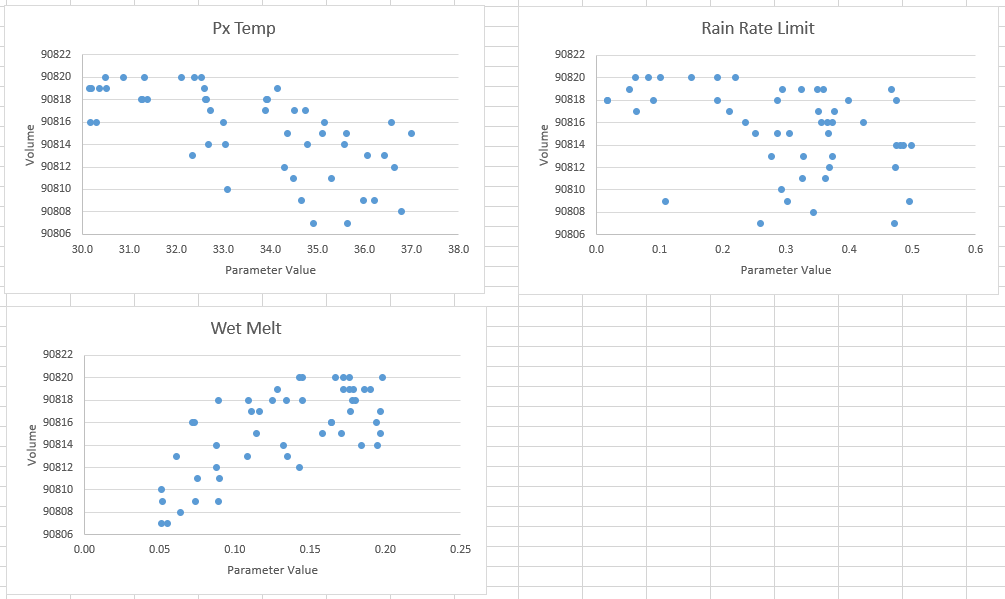
- Compute the Uncertainty Analysis and record your results in the “Max Outflow – Snow” and “Volume – Snow” worksheets.
Question: Compared to the runoff parameters, how much control do these snowmelt parameters have?
Using the values in the table above, more variability is seen in the peak discharges though the sensitivity is not as much as the baseflow parameters.
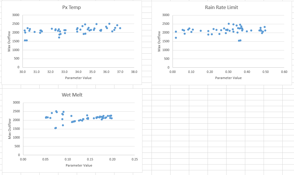
The volumes are fairly consistent and do not change significantly.
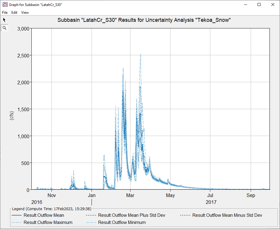
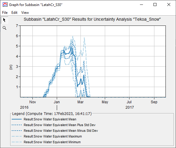
Question: Review the SWE uncertainty plot. What information can you glean from the graph that is not reflected in the snow parameter plots?
Looking over the Snow Water Equivalent plot, the snowmelt parameters have a significant affect on the snowpack build up and melt timing. This in turn has a direct impact on the hydrograph shape and timing which is not reflected in the peak and volume plots.
Question: Based on the sensitivity analyses above, if you were tasked with calibrating this watershed model, which parameters would you concentrate on the most?
Moving the surface parameters around isn’t likely to change the calibration much. GW 1 coefficient and GW 1 & 2 Fractions goes a long way to controlling peaks and the overall volume of the hydrograph. The three snowmelt parameters have a lot of power to control the overall timing and shape of the hydrograph, as well as the peak discharge.
Additional Task
If time allows, consider these additional tasks:
- Increase the number of Total Samples (i.e. from 50 to 250) and review the outputs. Does increasing the sampling provide some additional information that was missed with just sampling 50?
- Run an uncertainty analysis with a combination of parameters that you think is the most sensitive and see how much control you have over the resulting hydrograph for a reasonable range for each parameter. In DSS you can overlay the observed data with the hydrographs and the confidence limits.
