Download PDF
Download page Summarizing Student Results from the Basic HEC-HMS Final Project.
Summarizing Student Results from the Basic HEC-HMS Final Project
Last Modified: 2022-11-07 12:55:31.702
This tutorial demonstrates a newer option in HEC-HMS for defining parameter uncertainty using model calibration results from many different modelers.
Software Version
HEC-HMS version 4.11 beta 5 was used to create this example. You can open the example project with HEC-HMS 4.11 beta 5 or a newer version.
Have you ever wondered how different modelers might parameterize a model? Or, how could you incorporate different parameter sets (parameter set includes all parameters that make up the model) in an uncertainty analysis simulation? This tutorial demonstrates a newer option in HEC-HMS for defining parameter uncertainty using model calibration results from many different modelers. The same approach could be used to apply parameter sets from different flood events.
Introduction
The HEC-HMS team recently updated the Basic HEC-HMS training class, link here, and added a final project where students created a model application from scratch and then calibrated the model to the same flood event. You can download the data and work through the example model application here. There was some guidance on parameter adjustments and model metrics to strive for while calibrating the model. HEC-HMS does include an automated tool to adjust model parameter in order to calibrate the model to observations. However, an experience modeler still needs to formulate reasonable minimum and maximum parameter ranges and interaction between model parameters. Performing manual calibration is a good way to understand the model's response to parameter changes and is necessary for new modelers to become more familiar with impacts from individual model parameters.
Uncertainty in hydrologic modeling results can come from many sources, including boundary condition data, model structure, model parameters, initial conditions, and experience of the modeler. HEC-HMS includes an uncertainty analysis simulation type where modelers can define uncertainty information for initial conditions and model parameters. There are different methods in HEC-HMS for sampling parameter values, the simple distribution, regression with additive error, and the specified values sampling options. The specified values sampling option allows the modeler to choose a paired data table for each model parameter and the program will systematically cycle through the values in the paired data tables. The specified values sampling option maintains correlation between parameter values (as defined by the modeler in how the parameter value sample curves were created). For example, sample 1 will include all values in row 1 of the paired data tables, sample 2 will include all values in row 2 of the paired data tables, and so on. The specified values sampling option is a way to ensure reasonable model parameters, or a parameter set, is being used for each simulation in the uncertainty analysis. It is up to the modeler to correctly configure the paired data tables, which could be populated from model calibration to different historic flood events. The simple distribution and regression with additive error sampling methods can lead to unreasonable combinations of parameter values (HEC-HMS does not currently include an option to set up correlation between parameters when using sampling). For example, a low constant loss rate and Clark storage coefficient might be sampled and both values might be reasonable; however, the combination of lower values for both parameters can lead to an unrealistic model.
The goal of this tutorial is to:
- Show the range in hydrologic modeling parameters from different modelers;
- Demonstrate how the HEC-HMS uncertainty analysis simulation run type can be configured with the specified values sampling option.
Note
The procedure followed in this tutorial is not typical of hydrologic modeling studies. One goal is to demonstrate tools available tools in HEC-HMS. The specified values sampling method could be a helpful option if your study requires quantification of parameter uncertainty.
Model Application
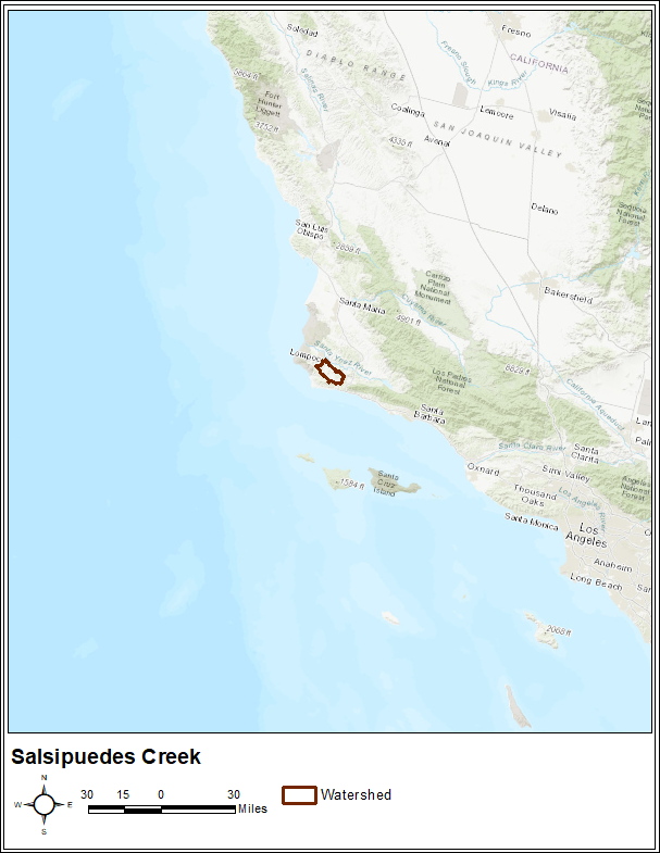
The project watershed is located upstream of the USGS stream gage(11132500) at Salsipuedes Creek near Lompoc, CA stream gage (11132500). Multi-Radar Multi-Sensor (MRMS) gridded precipitation was used for this February 2017 flood event. The Gridded Data Import tool (available from File | Import | Gridded Data | Importer) was used to convert the MRMS data to HEC-DSS format records. Fifteen minute streamflow data was gathered from the USGS.
Students Results
Most of the student modelers were new to HEC-HMS and hydrologic modeling. The spread in model parameters and calibration metrics is likely higher than would be expected from more experienced hydrologic modelers. The table below shows model parameters and calibration metrics from 62 students. The Nash-Sutcliff Efficiency score was greater than 0.9 and the percent bias in runoff volume was less than 15 percent across all models. Each parameter set, or model, was able to reproduce the runoff response from the intense precipitation event that occurred in February of 2017.
There was a limited amount of time students had for the workshop. The students were told to focus on peak flow and the Nash-Sutcliffe Efficiency score first before focusing on runoff volume. The more sensitive parameters to modeling peak flow are the constant loss rate and Clark storage coefficient. These two parameter do have some interaction with one another on the computed peak flow. For example, a smaller constant loss rate could be offset by a larger storage coefficient value. Notice the variability in these two model parameters from the student results. There is also some interaction between the linear reservoir baseflow parameters and the surface runoff storage coefficient. You could attempt to model the runoff response with mostly baseflow, or interflow by using a larger constant loss rate and smaller groundwater 1 and groundwater 2 coefficients; however, the figure below show baseflow/interflow is a relatively small contribution in the runoff response in this watershed, which makes it easier when determining realistic groundwater 1 and groundwater 2 fractions.

| Student Model | Initial Deficit (in) | Constant Loss Rate (in/hr) | Percent Impervious Area (%) | Time of Concentration (hr) | Storage Coefficient (hr) | GW 1 Fraction | GW 1 Coefficient (hr) | GW 1 Steps | GW 2 Fraction | GW 2 Coefficient (hr) | GW 2 Steps | Nash-Sutcliffe Efficiency Score | Percent Bias in Runoff Volume |
| 1 | 0.6 | 0.15 | 0 | 3 | 2.5 | 0.2 | 5 | 2 | 0.1 | 90 | 1 | 0.95 | 4.27 |
| 2 | 0.5 | 0.16 | 0 | 3.5 | 2.2 | 0.1 | 9 | 1 | 0.15 | 30 | 1 | 0.96 | 1.51 |
| 3 | 0.4 | 0.14 | 10 | 2 | 3 | 0.1 | 9 | 1 | 0.2 | 90 | 2 | 0.96 | 9.83 |
| 4 | 0.9 | 0.2 | 10 | 5.5 | 0.6 | 0.1 | 13.8 | 1 | 0.2 | 46 | 1 | 0.97 | 2.30 |
| 5 | 1 | 0.155 | 0 | 2.25 | 2.25 | 0.2 | 9 | 1 | 0.2 | 30 | 1 | 0.97 | 10.79 |
| 6 | 1 | 0.14 | 0 | 2.5 | 2.5 | 0.2 | 13.8 | 1 | 0.1 | 46 | 1 | 0.96 | 2.04 |
| 7 | 1 | 0.25 | 0 | 2.64 | 2 | 0.45 | 5 | 1 | 0.05 | 10 | 1 | 0.96 | 9.23 |
| 8 | 0.9 | 0.1 | 0 | 2.5 | 3.5 | 0.2 | 106 | 2 | 0.2 | 139 | 2 | 0.91 | -4.77 |
| 9 | 0.6 | 0.15 | 0 | 2 | 2.5 | 0.2 | 10 | 1 | 0.2 | 150 | 1 | 0.98 | 9.12 |
| 10 | 0.75 | 0.14 | 0 | 3 | 2.5 | 0.1 | 15 | 1 | 0.15 | 90 | 1 | 0.96 | -3.33 |
| 11 | 0.4 | 0.17 | 0 | 2 | 2 | 0.1 | 13.8 | 1 | 0.15 | 46 | 1 | 0.98 | -4.84 |
| 12 | 0.8 | 0.12 | 0 | 2.5 | 2.5 | 0.3 | 30 | 1 | 0 | 167 | 2 | 0.96 | 11.32 |
| 13 | 1 | 0.15 | 0 | 2.7 | 2.7 | 0.2 | 7.1 | 1 | 0.1 | 70 | 1 | 0.95 | -1.60 |
| 14 | 0.9 | 0.14 | 0 | 4 | 2 | 0.15 | 75 | 1 | 0.3 | 200 | 1 | 0.93 | -0.51 |
| 15 | 0.6 | 0.16 | 0 | 2.5 | 2.5 | 0.2 | 12.8 | 1 | 0.15 | 95 | 1 | 0.98 | 5.69 |
| 16 | 0.8 | 0.15 | 0 | 3.5 | 2.2 | 0.1 | 9 | 1 | 0.1 | 35 | 2 | 0.95 | -10.29 |
| 17 | 0.75 | 0.21 | 0 | 1 | 2.8 | 0.2 | 2.5 | 1 | 0.2 | 5 | 2 | 0.97 | 5.67 |
| 18 | 0.6 | 0.15 | 0 | 2 | 2 | 0.16 | 13.8 | 1 | 0.16 | 46 | 1 | 0.98 | 8.49 |
| 19 | 0.8 | 0.14 | 1 | 3.5 | 2.3 | 0.1 | 15 | 1 | 0.2 | 90 | 1 | 0.94 | 1.52 |
| 20 | 0.7 | 0.2 | 0 | 2.2 | 2.2 | 0.18 | 7 | 1 | 0.18 | 21 | 1 | 0.98 | 2.24 |
| 21 | 0.9 | 0.175 | 0 | 3.5 | 1.6 | 0.2 | 7 | 1 | 0.15 | 24 | 3 | 0.97 | 0.05 |
| 22 | 0.7 | 0.11 | 0 | 2.1 | 4 | 0.1 | 10 | 1 | 0.1 | 30 | 1 | 0.91 | 6.00 |
| 23 | 0.86 | 0.25 | 0 | 3 | 1.6 | 0.4 | 4 | 1 | 0.6 | 80 | 5 | 0.98 | -0.57 |
| 24 | 0.49 | 0.17 | 0 | 3 | 2 | 0.2 | 14 | 1 | 0.8 | 60 | 5 | 0.98 | -2.34 |
| 25 | 0.9 | 0.15 | 0 | 2.25 | 2.25 | 0.2 | 15 | 1 | 0.1 | 90 | 1 | 0.98 | 0.01 |
| 26 | 1 | 0.16 | 0 | 2 | 2 | 0.2 | 13.5 | 1 | 0.4 | 300 | 1 | 0.98 | -10.70 |
| 27 | 0.5 | 0.15 | 0 | 2.3 | 2.3 | 0.1 | 13.8 | 2 | 0.9 | 92 | 3 | 0.98 | 1.88 |
| 28 | 1.5 | 0.1 | 0 | 1.75 | 2.75 | 0.1 | 85 | 1 | 0.9 | 200 | 1 | 0.91 | 11.84 |
| 29 | 1 | 0.11 | 0 | 3.1 | 2.8 | 0.3 | 51 | 2 | 0.7 | 162 | 3 | 0.91 | 1.99 |
| 30 | 1 | 0.2 | 0 | 2.5 | 1.8 | 0.3 | 8 | 1 | 0.7 | 620 | 1 | 0.97 | 6.48 |
| 31 | 0.3 | 0.16 | 0 | 3 | 2.1 | 0.1 | 8 | 1 | 0.05 | 16 | 2 | 0.97 | -13.73 |
| 32 | 0.7 | 0.15 | 0 | 3.4 | 2 | 0.25 | 10 | 2 | 0.3 | 6 | 40 | 0.96 | -0.30 |
| 33 | 0.8 | 0.17 | 0 | 3.9 | 1.2 | 0.1 | 13.8 | 3 | 0.3 | 48 | 2 | 0.95 | -0.19 |
| 34 | 0.5 | 0.16 | 0 | 4.4 | 1.7 | 0.2 | 15 | 1 | 0.8 | 300 | 2 | 0.94 | -0.22 |
| 35 | 0.7 | 0.13 | 0 | 3.5 | 2.7 | 0.1 | 50 | 1 | 0.18 | 165 | 1 | 0.93 | -2.61 |
| 36 | 0.8 | 0.15 | 0 | 2.3 | 2.3 | 0.2 | 27.84 | 1 | 0.2 | 92.81 | 1 | 0.98 | 8.96 |
| 37 | 0.6 | 0.21 | 0 | 2 | 1.7 | 0.27 | 25 | 1 | 0.1 | 40 | 1 | 0.93 | 1.73 |
| 38 | 0.5 | 0.12 | 0 | 2.5 | 2.91 | 0.1 | 13.8 | 2 | 0.1 | 80 | 2 | 0.96 | -0.86 |
| 39 | 0.8 | 0.24 | 0 | 4 | 1.8 | 0.4 | 3 | 1 | 0.1 | 50 | 1 | 0.96 | 13.20 |
| 40 | 0.6 | 0.17 | 0 | 2.8 | 2.4 | 0.2 | 10 | 1 | 0.03 | 50 | 2 | 0.97 | -9.05 |
| 41 | 0.58 | 0.18 | 0 | 2.9 | 1.9 | 0.14 | 7.5 | 1 | 0.18 | 30 | 1 | 0.98 | 1.92 |
| 42 | 1 | 0.14 | 0 | 3 | 2.2 | 0.2 | 40 | 1 | 0.1 | 80 | 1 | 0.96 | -1.39 |
| 43 | 0.9 | 0.19 | 0 | 3 | 2 | 0.3 | 6 | 1 | 0.25 | 80 | 3 | 0.97 | 0.71 |
| 44 | 0.75 | 0.25 | 0 | 4.5 | 1 | 0.25 | 2 | 1 | 0.2 | 15 | 1 | 0.97 | 6.34 |
| 45 | 1.15 | 0.14 | 0 | 2.1 | 2.6 | 0.2 | 13.8 | 1 | 0.1 | 13.8 | 1 | 0.96 | -0.75 |
| 46 | 0.7 | 0.17 | 0 | 2.6 | 2.2 | 0.14 | 6.6 | 1 | 0.16 | 22 | 1 | 0.98 | 0.32 |
| 47 | 0.8 | 0.16 | 0 | 1.9 | 2.5 | 0.02 | 13.8 | 1 | 0.2 | 46 | 1 | 0.98 | -11.02 |
| 48 | 0.3 | 0.15 | 0 | 2.7 | 2.7 | 0.1 | 13.8 | 1 | 0.1 | 46 | 1 | 0.97 | -4.03 |
| 49 | 0.96 | 0.16 | 0 | 2.55 | 2 | 0.1 | 13.8 | 1 | 0.23 | 49.5 | 1 | 0.98 | -0.17 |
| 50 | 1 | 0.23 | 0 | 5.5 | 1 | 0.3 | 2.85 | 1 | 0.2 | 20 | 1 | 0.94 | 11.69 |
| 51 | 0 | 0.15 | 0 | 2.5 | 2.5 | 0.1 | 7.5 | 1 | 0.1 | 25 | 1 | 0.97 | -0.60 |
| 52 | 0 | 0.14 | 0 | 1.9 | 2.5 | 0.35 | 300 | 1 | 0.1 | 150 | 1 | 0.98 | -0.39 |
| 53 | 1 | 0.2 | 5 | 2.6 | 1.8 | 0.2 | 6 | 1 | 0.2 | 60 | 1 | 0.98 | 5.17 |
| 54 | 0.9 | 0.15 | 0 | 1.5 | 2.5 | 0.15 | 13.8 | 1 | 0.15 | 46 | 1 | 0.99 | 1.21 |
| 55 | 0.4 | 0.14 | 0 | 3 | 2.5 | 0.1 | 7.5 | 1 | 0.1 | 25 | 1 | 0.96 | -0.28 |
| 56 | 0.68 | 0.13 | 0 | 2.7 | 2.7 | 0.2 | 50.3 | 2 | 0.1 | 167.7 | 1 | 0.96 | -1.93 |
| 57 | 1 | 0.15 | 0 | 2.5 | 2.5 | 0.2 | 13.8 | 1 | 0.2 | 70 | 2 | 0.97 | 0.69 |
| 58 | 0.8 | 0.26 | 0 | 4.4 | 0.5 | 0.5 | 8 | 1 | 0.01 | 80 | 1 | 0.95 | 13.24 |
| 59 | 1.1 | 0.2 | 0 | 1.7 | 1.7 | 0.2 | 5 | 1 | 0.2 | 1 | 35 | 0.96 | -0.62 |
| 60 | 1 | 0.15 | 0 | 4 | 2 | 0.15 | 13.9 | 1 | 0.15 | 46.3 | 1 | 0.92 | -1.02 |
| 61 | 0.2 | 0.13 | 0 | 3.1 | 3.1 | 0.1 | 13 | 1 | 0.1 | 32 | 1 | 0.92 | 4.50 |
| 62 | 0.5 | 0.18 | 0 | 2.5 | 2 | 0.3 | 15 | 1 | 0.1 | 46 | 2 | 0.98 | 11.40 |
Uncertainty Analysis for the 2017 Event
The uncertainty analysis simulation was used to visualize results from all 62 models without setting up 62 separate basin models and simulation runs. Below are the steps followed to create the uncertainty analysis simulation and view results.
- Create Parameter Value Samples paired data curves for each of the eleven parameters that were varied by the students. The figure below shows the Component Editor for the Constant Loss Rate parameter value sample curve.

The figure below shows the first 12 constant loss rate values, from the first 12 rows in the students results table. It was important to make sure the same parameter set occupied the same row number across all parameter value sample curves. For example, parameters from model 1 occupied row one in all eleven parameter value sample curves. You do not want to mix parameters from models as this could result in an unrealistic parameter sets / models.
- An uncertainty analysis was created and named Uncertainty Feb_2017. As shown below, a basin model and meteorologic model were selected, a simulation time window and time-step were set, and then the total number of samples was set to 62 since there were 62 different parameter sets. The Seed Value was not used in this uncertainty analysis since only the specified value sampling option was used. With this sampling method, HEC-HMS starts with values in row 1 and cycles through all values in the parameter value sample paired data curves. The program will start over at row 1 if the number of samples exceeds the values in the paired data table.

- Eleven parameters were added to the uncertainty analysis.

Each parameter was linked to one of the parameter value sample curves. The figure below shows where parameter 1 was linked to parameter values samples for the Clark storage coefficient.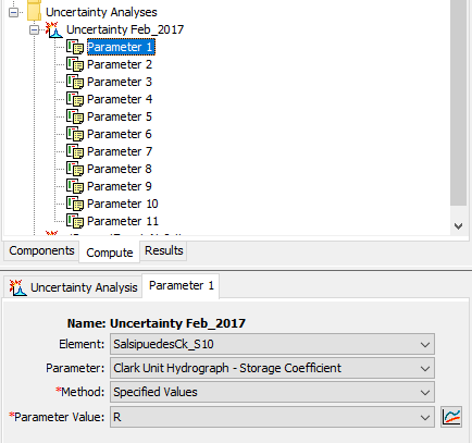
- By default, the uncertainty analysis does not save results from the simulation. The modeler must choose which results to save. The Outflow at the outlet element was saved.

The uncertainty analysis simulation was computed and results were viewed from the Results tab of the Watershed Explorer. The figure below shows the default plot from HEC-HMS, it includes the average, plus/minus one standard deviation, minimum, and maximum hydrographs.

You can also access results for each sample from the simulation DSS file. The figure below shows all 62 hydrographs plotted on top of one another; each hydrograph was generated by one of the parameter sets (models) in the students results table. You could generate the same results by setting up 62 different basin models and simulation runs in HEC-HMS; however, the uncertainty analysis is much quicker.

Note
HEC-HMS has an option to turn off writing notes and warnings to the message window and the output log file (see the Messages Table in the Program Settings editor). An uncertainty analysis with 1,000s of samples can generate a large amount of messages.