Creating Variable Clark Transform Method Parameters using the 2D Diffusion Wave Transform Method

CoyoteCreek.zip

HEC-HMS 4.7 beta 2 was used to create this tutorial.

Introduction

The purpose of this tutorial is to show how the new 2D Diffusion Wave transform method can be used to create relationships between excess precipitation and the Clark unit hydrograph parameters. One assumption with the applications of unit hydrograph transform methods is that the runoff response is linear with the magnitude of precipitation (2 units of excess precipitation generates a runoff response that is 2 times larger than the runoff response from 1 unit of precipitation). In natural watersheds, runoff response is not linear. As precipitation rates increase, channel velocities increase and natural storage in channels and floodplains change as well. The non-linear runoff response is one reason guidance states that models should be calibrated to the magnitude of event used in predictive simulations. In some applications, it is necessary to use a model to predict the runoff response for events much larger than those even available for calibration. In these cases, model parameters could be modified, or alternative models used.

The HEC-HMS team added an option to the Clark unit hydrograph method that allows modelers to vary the time of concentration and storage coefficient parameters based on excess precipitation intensity. Developing the relationship between time of concentration and storage coefficient parameters and excess precipitation can be challenging. Historical storm events could be used if there were several storm events with varying precipitation intensities. Another option is to use numerical models, like the 2D Diffusion Wave transform method, that includes the physics of overland flow and would be able to model the non-linear change in runoff response as precipitation rates increase.

This tutorial shows how to use the new 2D Diffusion Wave model in HEC-HMS (the same code in HEC-RAS), to create the variable parameter relationships for the Clark unit hydrograph method. The variable Clark method has application for studies where many, many simulations will be computed with moderate to extreme precipitation rates to evaluate uncertainty and parameter sensitivity on a watershed's runoff response. It might not be possible to run many events through the 2D Diffusion Wave transform solution in an uncertainty analysis. The variable Clark option can capture the non-linearity in runoff response while computing in a fraction of the time.

Further Information

Regression equations that can be used to estimate Variable Clark unit hydrograph parameters throughout the state of California have been developed and are detailed here: Variable Clark Unit Hydrograph Parameter Regression Equations for California.  A tutorial detailing their usage can be found here: Applying the Variable Clark Unit Hydrograph Method.

Watershed Description

The area modeled in this tutorial is part of the Coyote Creek watershed in Northern California. See the following tutorial for information about the watershed and how the HEC-HMS model was developed - Comparing HEC-HMS Discretization and Transform Options. In summary, an HEC-HMS model was developed for part of the Coyote Creek watershed, the upper 109 square miles. Observed precipitation and flow data were used to calibrate the model. The subbasin element was configured to use the Deficit and Constant loss method, 2D Diffusion Wave transform method, and the Linear Reservoir baseflow method. The 2D unstructured mesh had 18,512 grid cells. As described below, the 2D model was used to create variable Clark parameter relationships.

The 2D model simulation takes 7 minutes to run the two-day window for the December 1982 event. The variable Clark model takes 1 seconds to run the same time window.

Step 1: Calibrate the 2D Model

A model must be calibrated to observations in order to be used for future prediction. This is true for models that include the physics of the natural processes as well as conceptual and empirical models. When developing the Coyote Creek HEC-HMS 2D model, the infiltration, transform, and baseflow parameters were adjusted, within reason, to improve the performance of the model to the 1982 event. The following figure shows results from the December 22, 1982 flood event. The Nash-Sutcliffe metric was 0.89 and the percent bias in runoff volume error was 3.8 percent. Timing of the runoff hydrograph was improved by adjusting the surface roughness parameters while magnitude of peak flow and volume of the runoff hydrograph were improved by adjusting loss and baseflow parameters.

Ideally more than one flood event would be used to calibrate the model, and additional events would be used to validate the model. If you download the example project, the calibrated basin model is named CoyoteCreek_2D and the simulation run is named 1982_2D.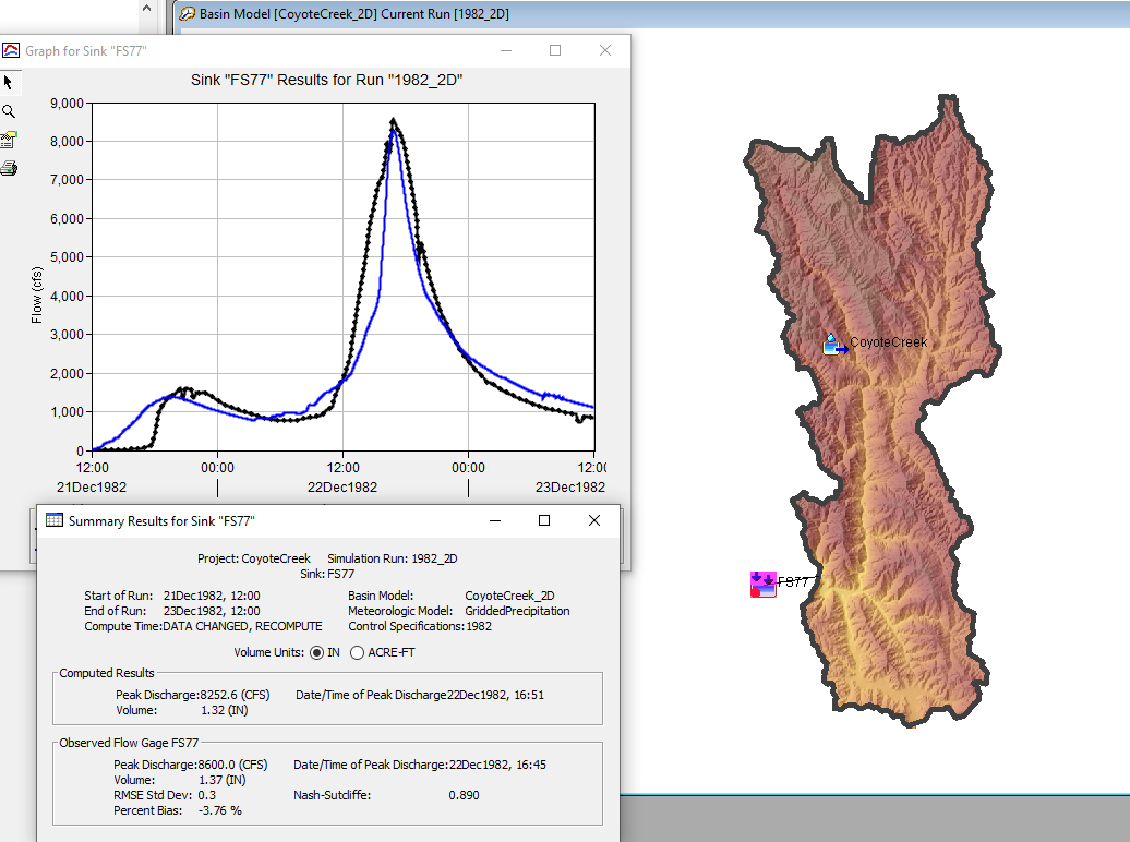

Step 2: Apply Varying Units of Precipitation to the Calibrated 2D Model

Once the basin model was calibrated, a series of hypothetical precipitation "events" were applied to the basin model. Each event contained different precipitation intensities. The precipitation intensities included 0.25 inch/hour, 0.5 inch/hour, 1.0 inch/hour, 2.0 inches/hour, and 4.0 inches/hour. Five precipitation gages were added to the project, one for each precipitation intensity. The figure below shows a portion of the Watershed Explorer with the five precipitation gages and the Component Editor shows a plot of the 1 inch/hour precipitation gage. As shown below, there was an antecedent precipitation of 0.5 inches/hour used in all five gages. This antecedent precipitation was used to fill in any low spots, or pits, in the terrain prior to the main precipitation event. Five meteorologic models were created, each meteorologic model used one of the five precipitation gages.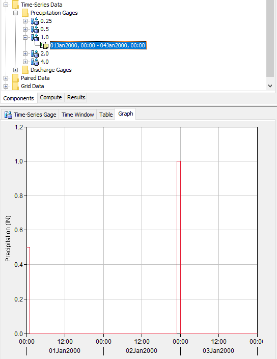

A copy of the calibrated basin model was made and named CoyoteCreek_2D_peaking. The Loss and Baseflow methods were set to None. The only hydrologic process turned on was the 2D Diffusion Wave transform method. Five simulations were created for the hypothetical simulations. The simulation time window for the five hypothetical simulations was 01 January 2000 at hour 00:00 though 06 January 2000 at hour 00:00. The following table contains the basin and meteorologic model combinations for the five hypothetical storms.

The following figure shows results from the simulation where the main precipitation was 1 inch/hour. Notice the precipitation depth is a little larger than 0.016 inches in the plot. The simulation time-step was 1 minute, 1 inch/hour divided by 60 minutes is 0.0167 inches. The meteorologic model applied 0.0167 inches per minute for a 1-hour period. The resulting hydrograph is the runoff response from 1 inch of precipitation applied to the subbasin element. The subbasin element only had the 2D Diffusion Wave transform option turned on, so only surface routing computations were performed during the simulation.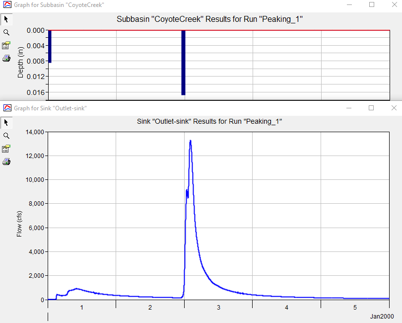

The following figure shows a comparison of the runoff hydrograph from three of the hypothetical simulations. The hydrographs do not represent unit hydrographs since they have not been normalized to one inch of precipitation. Notice how the time of the peak flow shifts as the precipitation intensity increases.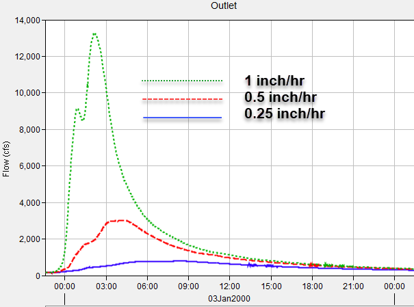

Step 3: Calibrate the Clark Model to the 2D Model Results

After running the hypothetical precipitation events with the 2D Diffusion Wave transform model, the next step was to use HEC-HMS to identify Clark parameters, time of concentration and storage coefficient, that could reproduce results from the 2D solution. Five Discharge gages were created and linked to results from the hypothetical simulations in step 2. The following figure shows the 2DComputed_1 discharge gage is linked to results from the Peaking_1 simulation. Results from the 2D transform simulations were used as observed flow in the Clark unit hydrograph simulations (the discharge gages were linked to the Outlet sink element).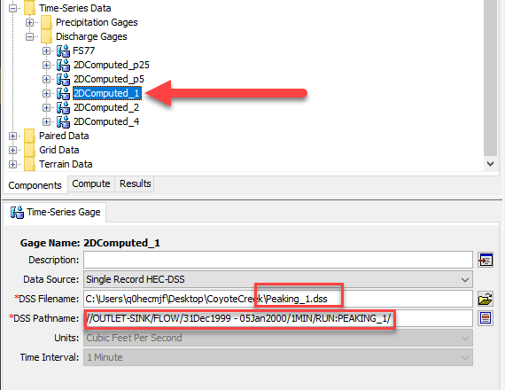

The CoyoteCreek_2D_peaking basin model was copied, and the transform method was changed from 2D Diffusion Wave to Clark Unit Hydrograph. Four additional copies were created. Five copies were needed in order to identify a separate set of Clark parameter for each of the hypothetical precipitation simulations in step 2. Five simulations were created as well that combined the Clark unit hydrograph basin models and the hypothetical meteorologic models. The following table shows the basin model, meteorologic model, and simulation run names for the Clark unit hydrograph simulations.

The Clark unit hydrograph parameters were adjusted for each hypothetical precipitation event to find a combination of time of concentration and storage coefficient that reproduced the 2D transform results. The following figure shows the results from the Clark simulation where the time of concentration and storage coefficient were adjusted to match results from the 2D simulation that had 1 inch of precipitation. A time of concentration of 3 hours and a storage coefficient of 3.5 hours was found to reproduce results from the 2D Diffusion Wave simulation.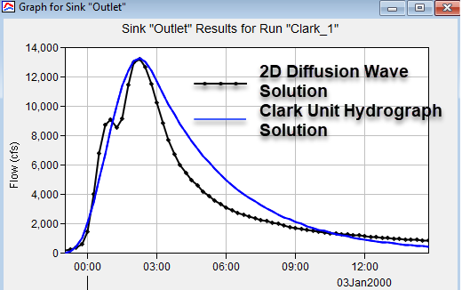

The following figure shows the results from the Clark simulation where the time of concentration and storage coefficient were adjusted to match results from the 2D simulation that had 0.5 inch of precipitation. A time of concentration of 4.5 hours and a storage coefficient of 9.0 hours was found to reproduce results from the 2D Diffusion Wave simulation.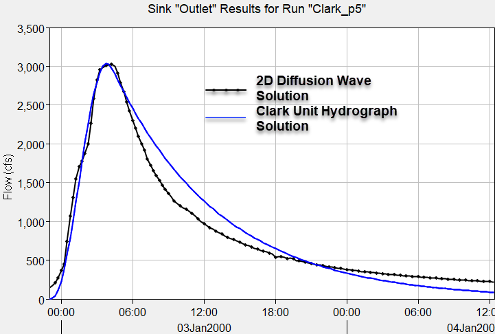

The following table contains results from the five Clark unit hydrograph simulations. Notice how the time of concentration and storage coefficient values decrease as the precipitation intensity increases.

When the Clark, Snyder, and SCS synthetic unit hydrographs are selected for a subbasin element, HEC-HMS will compute the unit hydrograph and save the unit hydrograph as a paired data record to the simulation DSS file. The following figure shows the records in the Clark_1.dss file. The unit hydrograph is saved to a record with a C-part pathname of FLOW-UNIT GRAPH.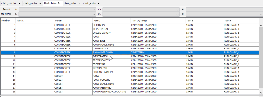

The following figure shows all five unit hydrographs from the five hypothetical precipitation simulations (the volume of runoff from each of the hydrographs shown below is 1-inch). Notice the non-linear behavior in the unit hydrographs. The time of peak flow become much shorter and the shape of the unit hydrograph becomes much more peaked, runoff is concentrated over a shorter period. In summary, these Clark unit hydrographs were created for specific precipitation intensity values and were developed by adjusting Clark unit hydrograph parameters to match results from a calibrated 2D Diffusion Wave transform model.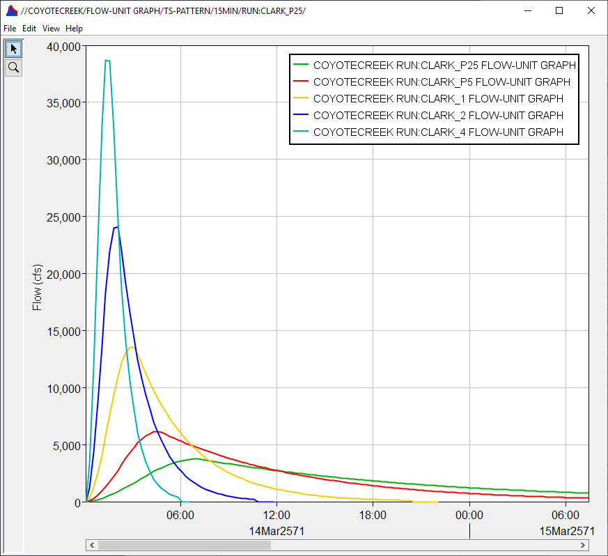

Step 4: Develop the Variable Clark Relationship

The figure below shows the Variable Parameter Clark Transform Component Editor. The modeler must define the Time of Concentration and Storage Coefficient for an Index Excess precipitation rate. The following figure shows an index excess precipitation rate of 1 inch/hour was entered; therefore, the time of concentration and storage coefficient parameters should be appropriate for an excess precipitation rate of 1 inch/hour. The modeler must also define a Concentration curve and a Storage curve. Both curves are Percentage Curve (%X and %Y). The concentration curve has an independent variable of percent Index Precipitation and the dependent variable is percent Time of Concentration. The storage curve has an independent variable of percent Index Precipitation and the dependent variable is percent Storage Coefficient.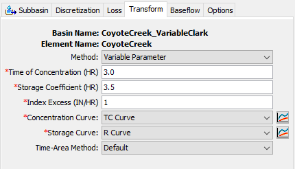

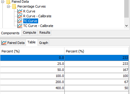
The following table shows the percentage curves for time of concentration and storage coefficient. The percentages are keyed from values for the index precipitation rate of 1 inches/hour. Percentage curves were created for both time of concentration and storage coefficient. The values shown below were entered into percentage paired data tables. The following figure shows the Concentration percentage curve, it is named TC Curve in the example project.

Step 5: Calibrate the Variable Clark Relationship

To test the variable Clark parameters, the CoyoteCreek_2D basin model was copied and the copy was named CoyoteCreek_VariableClark. The transform method was changed to Clark Unit Hydrograph and the Variable Parameter option was selected within the subbasin Component Editor. As shown above, an index excess precipitation rate of 1 inch/hour was entered and so were the Time of Concentration, 3 hours, and Storage Coefficient, 3.5 hours, that were determined when calibrating the Clark model to the 2D results for a precipitation rate of 1 inch/hour. The Concentration and Storage curves created above were selected as well.

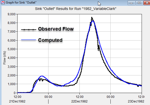
A simulation named 1982_VariableClark was created that combined the CoyoteCreek_VariableClark basin model, the GriddedPrecipitation meteorologic model, and the 1982 control specifications. Results from the simulation are shown below, the computed hydrograph does not match the magnitude and shape of the observed runoff hydrograph.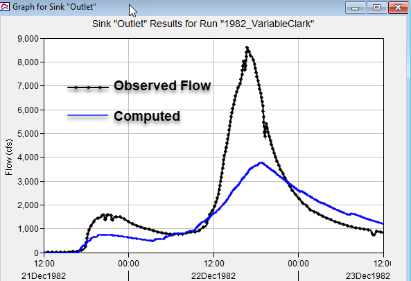

Why does the computed hydrograph not match the observed hydrograph? A calibrated 2D Diffusion Wave transform method was used to develop relationships between excess precipitation and the Clark time of concentration and storage coefficient parameters. However, the approach used does not mimic the variable nature of precipitation from natural flood events, like the event being modeled on December 22, 1982. The figure below shows the basin average precipitation for the December 22, 1982 event. The precipitation rate does not approach the 1 inch/hour rate, but there are six consecutive hours where the precipitation rate exceeds 0.2 inch/hour. During this extended period of precipitation, rainfall is falling onto a wet watershed. There is water flowing across the land surface in streams as precipitation is fall. This natural event is not the same as the hypothetical events used to derive the variable parameters; the event and results remind us that the time-invariance assumption used with the application of unit hydrographs has limitation. The main point here is that a unit of precipitation falling onto a watershed will respond differently with different antecedent conditions.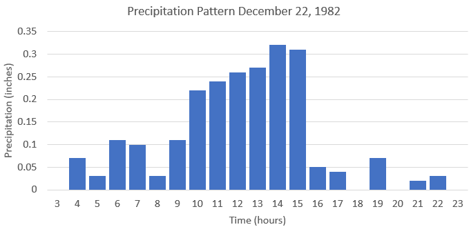

The variable time of concentration and storage coefficient percentage curves were adjusted to improve the model results for the 1982 event. In addition, the constant loss rate was reduced from 0.25 inches/hour from the 2D simulation to 0.16 inches/hour for the variable Clark simulation. The following table shows the updated concentration and storage curves.

The following figure shows the updated results after adjusting the variable time of concentration and storage coefficient curves and loss rate. The precipitation rates for the December 22, 1982 event only allow calibration of the lower end of the variable time of concentration and storage coefficient curves since the precipitation rate is less than 0.5 inch/hour. Events with higher precipitation intensities would be needed to improve the upper end of the variable parameter curves.

The approach and tools in this example provide a method for using unit hydrographs for a range of flood events. The most useful application for the variable Clark unit hydrograph method could be for extreme events (for those synthetic flood events that are larger than typical calibration data). The linearity assumption with unit hydrographs often leads modelers to arbitrarily adjust unit hydrograph parameters when applying models for simulating extreme floods. In the Coyote Creek example, the 2D Diffusion Wave simulations show the time of concentration decreases from 4.5 hours for an excess precipitation rate of 0.5 inch/hour to 2 hours for a excess precipitation rate of 2 inches/hour. The storage coefficient has a much more dramatic reduction (from 9 hours to 1.75 hours), which translates to a much faster responding hydrograph at higher precipitation rates. The information gathered from the 2D Diffusion Wave simulation can be used to inform the variable Clark unit hydrograph model which could then be used to quickly model the subbasin response to extreme events.