Download PDF
Download page Applying Gridded Precipitation to a Non-Georeferenced Project - Structured Discretization.
Applying Gridded Precipitation to a Non-Georeferenced Project - Structured Discretization
 Final_Gridded_Precip.zipFinal_Gridded_Precip.zip
This tutorial was updated on Sept 25, 2020 using HEC-HMS 4.7 Beta. The structured discretization method can be used instead of the *.mod file that was created by HEC-GeoHMS and HEC-HMS versions 4.4 - 4.6.1.
For creating a gridded boundary condition see Creating Gridded Boundary Conditions for HEC-HMS.
There are existing HEC-HMS models that can be updated and improved to utilize gridded precipitation and hydrologic methods. Many of these existing models are not georeferenced with coordinate system or projection information. These models often do not have background maps of the subbasins and reaches. When background maps of the subbasins and reaches are available the coordinate system information is often missing. These older models often use the lump approach for representing subbasins and hydrologic methods rather than the more useful gridded models, which allows the watershed to be represented in greater detail spatially.
In order to use gridded precipitation in the meteorological model and hydrologic methods in the basin model, the user must first georeference the basin model. When converting a lumped basin into a gridded basin, the user needs to process the terrain data for flow directions, and then generate either a structured or unstructured grid. The structured or unstructured grid specifies which grid cells are in each subbasin and the properties of each cell including location, area within the subbasin, distance to the subbasin outlet, and contain geospatial information about the grid.
This tutorial is designed to help the user of HEC-HMS learn how to apply a gridded precipitation dataset to a non-georeferenced project.
Overview
In this tutorial, you will perform three tasks to georeference existing subbasin and reach elements before generating a structured grid: 1) georeference the project, 2) process terrain information to create a flow direction grid, and 3) create a structured (SHG) grid for each subbasin.
Background
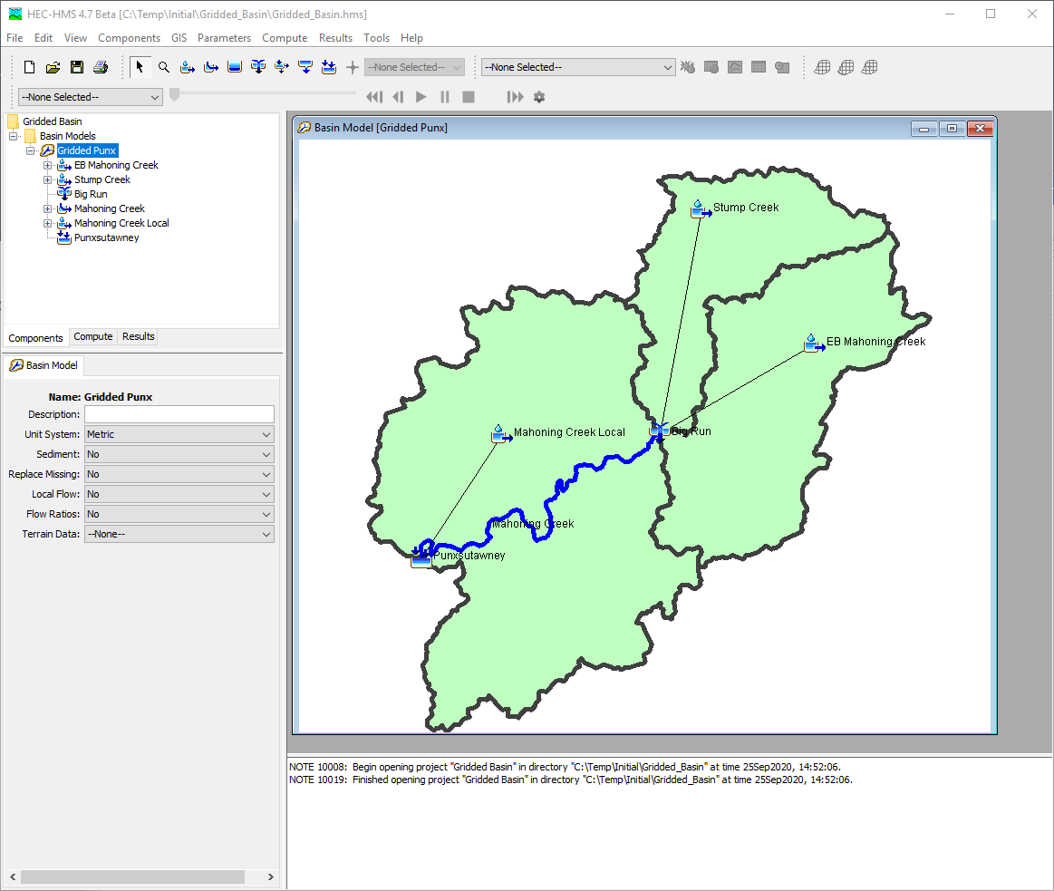
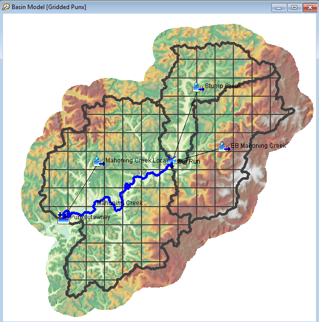
The Punxsutawney Watershed (400 km2) is part of the Allegheny River Basin located in western Pennsylvania, USA. Primary conveyance streams include: Stump Creek; East Branch Mahoning Creek; and Mahoning Creek. The confluence of Stump Creek and East Branch Mahoning Creek is located east of the enclave of Big Run. Mahoning Creek is downstream of the confluence.
A map of the watershed is shown below.
Task 1: Import and Georeference Subbasin and Reach Elements
The basin model was originally defined by delineating subbasins and river reaches using non-GIS tools, therefore, the basin model elements were not georeferenced. Starting with HEC-HMS version 4.3, there are tools to georeference existing subbasin and reach elements using the geospatial information in shapefiles.
The user can import subbasin and reach elements from shapefiles, or georeference existing HEC-HMS subbasin and reach elements. HEC-HMS uses the name attribute within the subbasin and reach shapefiles when importing information from shapefiles. The following steps shows how to georeference existing subbasin and reach elements.
- Double click the HEC-HMS icon
 to start the program. The main program window will appear.
 - To open an existing project, click File and select Open….
- The Open an Existing Project window will open; click Browse to open the Select Project File window.
- Navigate to the project directory and select the Gridded Basin.hms file.
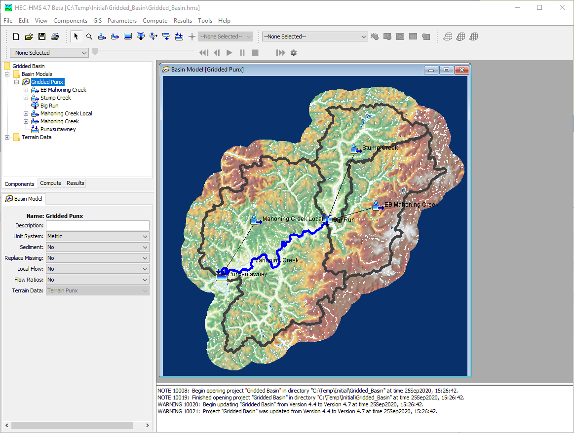
- Click the Select button and the existing project will open as shown below. Notice the basin model is not georeferenced because the elements are displayed as icons.

- The subbasin delineation is shown below. Subbasin and reach shapefiles have been created that contains an attribute with names that match the element names in the HEC-HMS basin model.

- Go to the GIS menu and choose the Georeference Existing Elements menu option.
- Choose the Subbasins element type and click the Next button.
- Navigate to the … \Gridded_Basin\maps directory and select the Basin Punx.shp file. Click Select. Click Next.
- Choose the name attribute field to set the subbasin element names. Click the Finish button.
- On the Coordinate System dialogue box, Click Select….
- Click Browse, Select the Basin Punx.prj file. Click Select Click Set. The coordinate system information should populate as shown below.

- Follow the previous steps and import the reach feature in the Reach Punx.shp file. The figure below shows the three subbasin elements and the one reach element that were imported from the two shapefiles.
- Right click on the Gridded Punx basin model name in the Watershed Explorer and choose the Resort Elements Hydrologically menu option. The elements in the Watershed Explorer should be ordered from upstream to downstream, as shown below.
Task 2: Load Terrain Dataset and Run the Preprocessing Steps
- Go to the Components menu and choose the Create Component menu option as shown below.

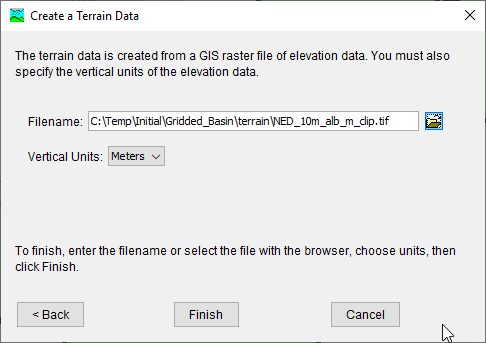
- Select Terrain Data, enter a Name of "Terrain Punx". Click Next as shown below.

- Navigate to the … \Gridded_Basin\terrain directory and select the file named NED_10m_alb_m_clip.tif. Change the vertical units to meters and click Finish as shown below.
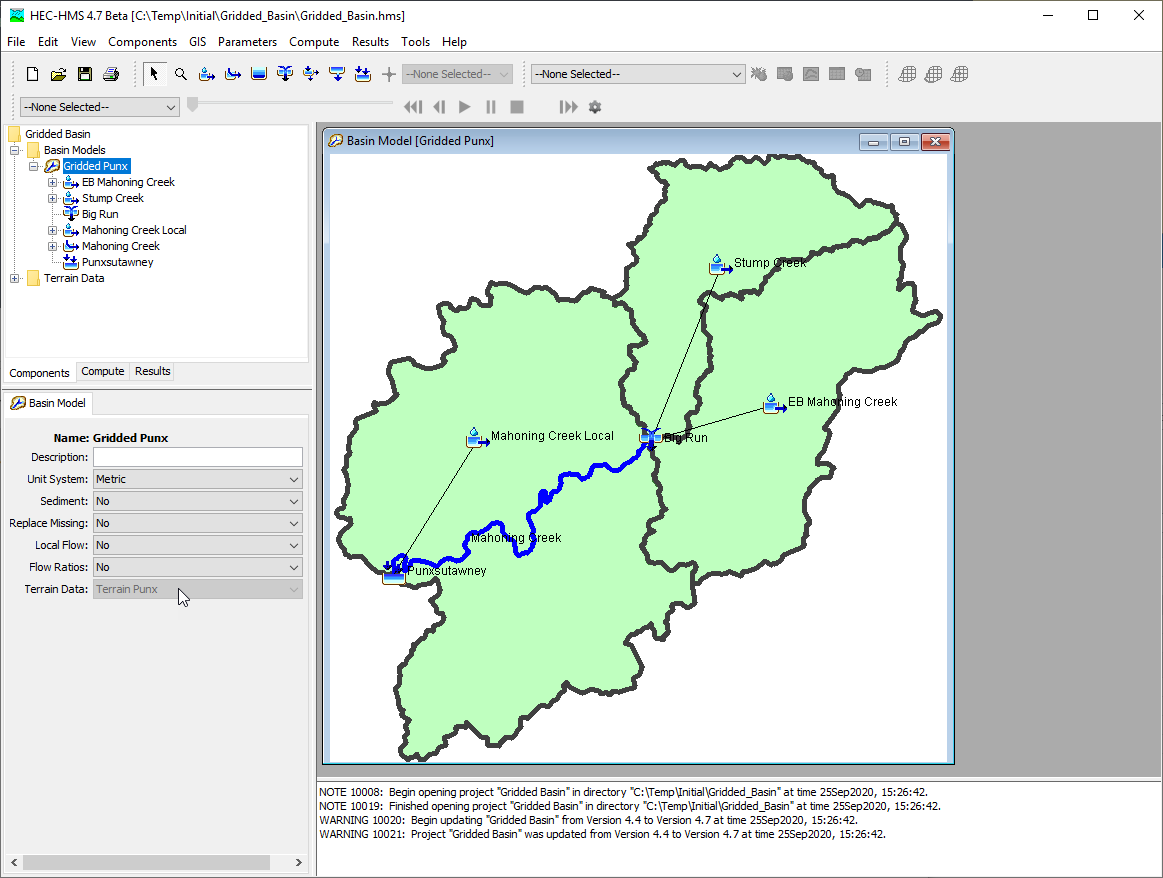
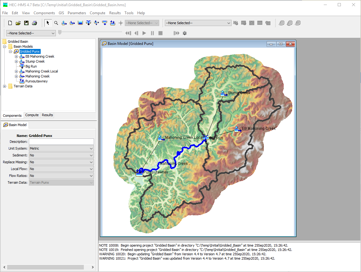
- After the terrain data has been added to the project, it can be associated to a basin model. Open the Gridded Punx basin model's Component Editor and then select Terrain Punx for the Terrain Data as shown in the two figures below. The terrain's coordinate system is read automatically from the Terrain Punx.tfw file.
- Select Terrain Data, enter a Name of "Terrain Punx". Click Next as shown below.
- The purpose of the next few steps is to perform drainage analysis on the terrain and produce a flow direction grid that will be needed later to create the grid cell file. Terrain data is a gridded representation of the watershed surface with elevation for each grid cell. This Preprocess Sinks step fills the sinks or depressions in the terrain so that the drainage analysis is possible. Go to the GIS Menu and choose the Preprocess Sinks menu option as shown below. The result of this step is a terrain without depressions, and a Sink Fill raster, as shown below.
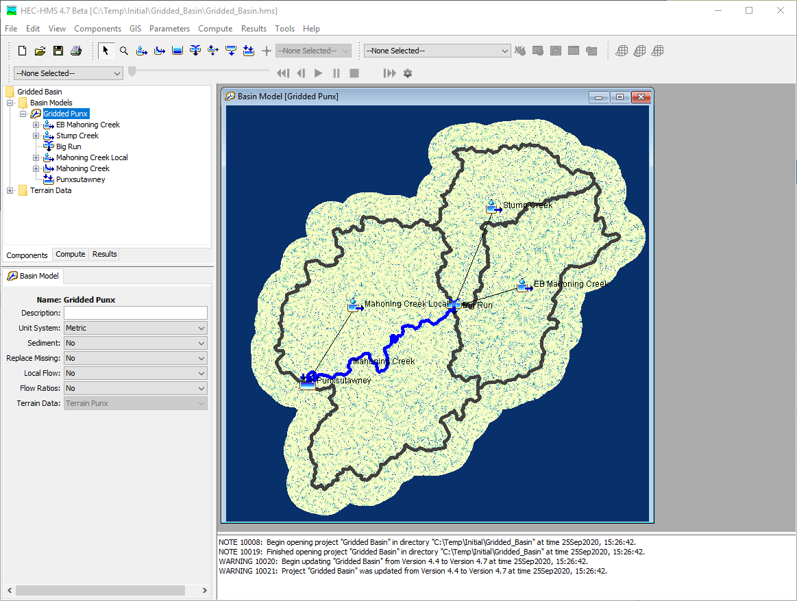
- Using the Sink Fill data from the previous step, the Preprocess Drainage step performs drainage analysis and produces the flow direction and flow accumulation data. Go to the GIS Menu and choose the Preprocess Drainage menu option as shown below.
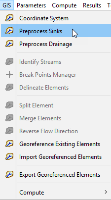
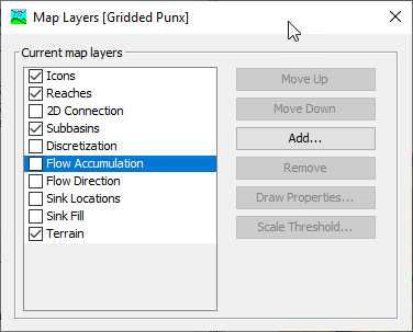
- This optional step shows how to turn off the visibility of map layers to speed up the map display. Go to the View Menu and choose Map Layers in the menu option. Uncheck the visibility for the Flow Accumulation, Flow Direction, Sink Locations, and Sink Fill layers as shown below.
Task 3: Create a Structured (SHG) Grid for each Subbasin
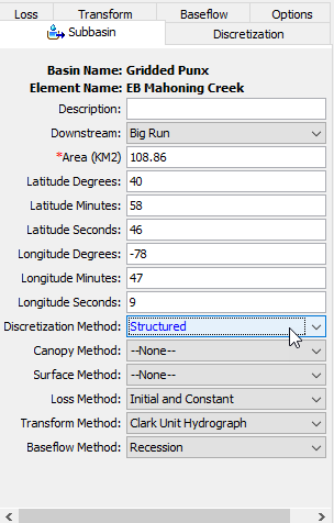
- The Discretization method must be selected for each subbasin element. By default, the "--None--" discretization method is selected. The none method means no gridded precipitation can be applied to the subbasin element and that none of the gridded canopy, surface, loss, and transform method can be selected. Only subbasin average methods can be used with the none discretization method. The Structured discretization method replaces the grid cell approach (*.mod file) that was available in previous versions of HEC-HMS. The structured discretization method lets the modeler choose between a grid in either the Standard Hydrologic Grid (SHG) or UTM grid projections, and the modeler can choose the grid cell size. Once the modeler chooses the grid type, SHG or UTM, and then the grid size, HEC-HMS automatically creates the grid and intersects the grid with the subbasin boundary. The figure below show the Structured discretization method selected for the EB Mahoning Creek subbasin. Choose the Structured discretization method for all three subbasin elements.
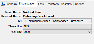
- Go to the Discretization tab in the Subbasin's Component Editor and make sure the SHG Projection is selected and that the Grid size is set to 2000 meters, as shown below. Do this for all three subbasins.
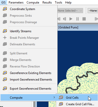
- Go to the GIS menu and select Compute→ Grid Cells as shown below.
- After the grid cells have been computed, open the Map Layers window and check the box next to Discretization. The 2000 meter SHG should be displayed in the basin model map as shown below.
The spatial information is saved in an *.sqlite file in the project directory. The *.sqlite file will be named using the basin model name. You can visualize the tabular data in this file using a tool like DB Browser. The geospatial information can be displayed in QGIS. Now that a structured grid has been developed for this basin model, gridded precipitation can be applied.