Download PDF
Download page Task 4: Creating an observed SWE time-series.
Task 4: Creating an observed SWE time-series
Return to Task 3: Normalizing Precipitation Data
Last Modified: 2024-08-28 16:08:37.008
HEC-HMS version 4.12 was used to create this example. You can open the example project with HEC-HMS v4.12 or a newer version.
The task is part of the Downloading, Importing, and Processing Gridded Data tutorial. You cannot continue with project files from Task 3: Normalizing Precipitation Data. Download new project files here:

Introduction
In this workshop you will use the HEC-HMS Gridded Data Import Wizard to import gridded SWE data. Then you will use the Grid-to-Point utility to create a daily average SWE time-series. Finally you will link the SWE data in HEC-HMS as an observed SWE time-series.
Download University of Arizona SWE data
There are two common sources of Snow Water Equivalent (SWE) data distributed with coverage for the conterminous United States: Snow Data Assimilation System (SNODAS) and University of Arizona (UA). Both provide a spatial SWE product and both are frequently applied as "observed" SWE in HEC-HMS, although both derive SWE by modeling the snow pack with observed inputs from meteorologic inputs, e.g. precipitation and temperature, in a similar manner to the snow pack modeling methods in HEC-HMS.
Download University of Arizona SWE data. The following link is an FTP site with NetCDF files: https://climate.arizona.edu/data/UA_SWE/
Download the UA_SWE_Depth_WY2017.nc file.
Import UA SWE data
Convert the data in NetCDF format to HEC-DSS using the Gridded Data Import Wizard.
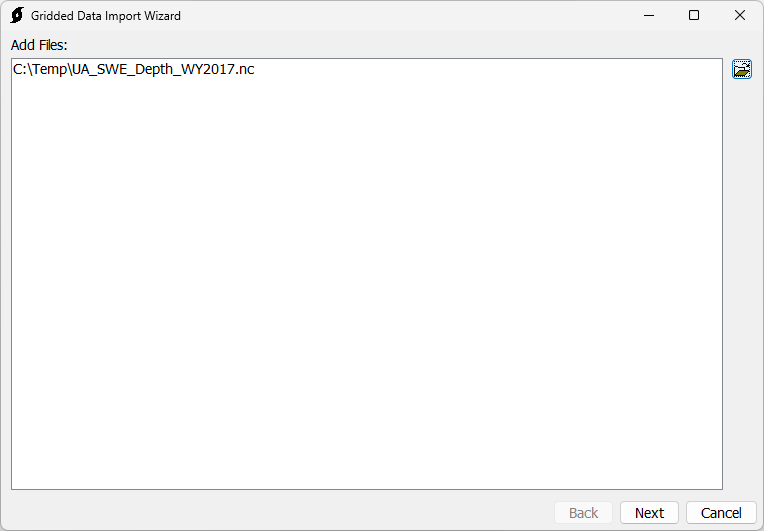
In HEC-HMS File | Import | Gridded Data | Importer to launch the Gridded Data Import Wizard.
On the first step of the wizard select the UA_SWE_Depth_WY2017.nc file.
On the second step of the wizard select the "SWE" variable for import.
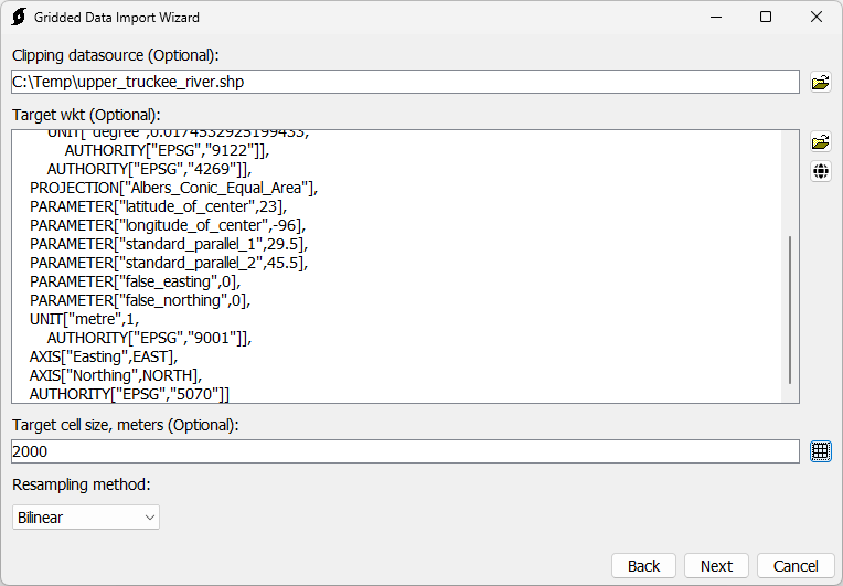
On the third step of the wizard specify resampling parameters:
- The Clipping datasource specifies the extent to which the data will be clipped to. Use the shapefile that was exported in Exporting a clipping shapefile.
- The Target WKT is the projection, in Well Known Text format, that the data will be projected to. Use the globe on the right to select the SHG projection.
- The Target cell size is the grid cell size that the data will be resampled to. Use the grid button on the right to select 2000 meters.
- The Resampling method is the method used to resample the data. Select the Bilinear resampling method.
On the fourth step of the wizard save the data to a file named UA_SWE.dss.
Click Next to import that data.
Convert UA SWE data to a time-series
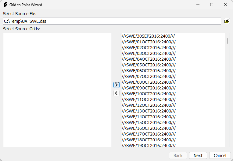
In HEC-HMS, from Tools | Data | Grid-to-Point, launch the Grid-to-Point Wizard.
In the first step of the wizard select the UA_SWE.dss file. Select all gridded records.
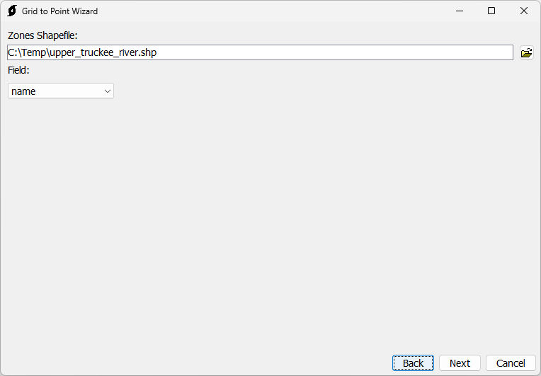
In the second step of the wizard, specify zonal statistics parameters:
- The Zones shapefile defines the geometries for which the zonal statistics will be calculated. Select the shapefile that was created in Export a clipping shapefile.
- The Field is the basis for the HEC-DSS pathname B-part for the HEC-DSS record that will be created. Select the name field.
On the third step of the wizard, write the time-series to the file <path to>/Upper_Truckee_River/data/Obs_Data.dss.
Set the F-part for the written record to "UA SWE".
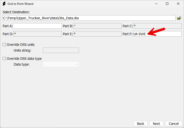
Click Next to proceed with the zonal statistics calculation.
Apply the SWE time-series as an Observed SWE time-series in HEC-HMS
Create a new SWE time series gage.
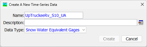
From Components | Create Component | Time-Series Data launch the Create A New Time-Series Data dialog.
Set the time-series data Name to UpTruckeeRv_S10_UA.
Set the Data Type to Snow Water Equivalent Gages.
In the Component Editor for the UpTruckeeRv_S10_UA time-series data data, set DSS Filename to <path to>/Upper_Truckee_River/data/Obs_Data.dss. Set the DSS Pathname to //UPTRUCKEERV_S10/SWE/01JAN2016 - 01JAN2017/1DAY/UA SWE/.

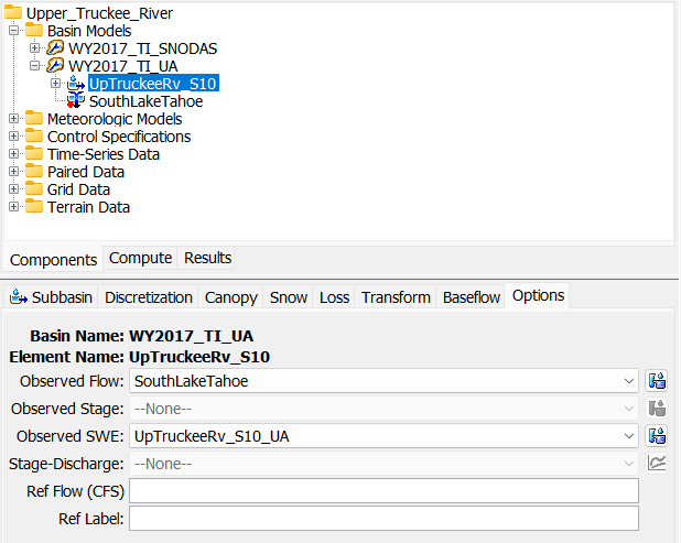
In the WY2017_TI_UA basin model component editor, Options tab, set the Observed SWE to UpTruckeeRv_S10_UA.
Run the WY2017_MRMS_UA simulation run.
Compare Observed SWE time-series from the WY2017_MRMS_UA and WY2017_MRMS_SNODAS simulations.

Notice the SNODAS and UA SWE have discrepancies but trend similar. It is important to remember these are modeled products and are not observations.
Summary
In this tutorial:
- University of Arizona SWE data was downloaded,
- the Gridded Data Import Wizard was used to import SWE data to HEC-DSS,
- the Grid-to-Point utility was used to extract a daily SWE time-series,
- and the daily SWE time-series was applied as an Observed time-series in HEC-HMS.
You can download final project files for this task here:
This concludes the Downloading, Importing, and Processing Gridded Data tutorial.