Download PDF
Download page Part 1: Importing Gridded Data.
Part 1: Importing Gridded Data
Last Modified: 2024-05-17 08:47:47.456
This workshop can be completed as part of the Workflows for Downloading, Importing and Manipulating Gridded Data or as a stand-alone activity.
HEC-HMS version 4.11-beta.10 was used to create this example. You can open the example project with HEC-HMS v4.11 or a newer version.
In this workshop, you will use HEC-HMS Gridded Data Import Wizard to import gridded SWE and temperature data and add the grids to the Upper Truckee River watershed model. Because grid data files often cover areas much larger than the footprint of the project, clipping these files to the watershed area can drastically reduce file size. The clipping extent file for the Truckee River watershed is provided below. The clipping shapefile can also be created in HMS by selecting GIS | Export Layers and selecting the Subbasins layer type. If you do so, be sure to buffer any polygon used for clipping by 1 to 2 miles (this can be done with GIS software).
Project files
Project Files

A note on data quality
The quality of gridded data will vary and should be assessed to ensure the information is suitable for the purpose of the model it is being applied to. Factors such as radar beam blockage and the distance from the radar station to the storm can affect the measurement of precipitation data. It is recommended that gridded data be compared to other data sources to determine if it is sufficient for use in a hydrologic model. For example, gridded precipitation can be compared to point gage data to check the magnitude and timing of a rain event. Programs like the HEC Meteorological Visualization Utility Engine (MetVue) make it easy to compare gridded data to point rainfall.
Importing gridded SWE data
Snowmelt is an important part of the hydrologic cycle in many watersheds. Snow water equivalent (SWE) represents the volume of liquid water available in the snowpack. You will download, import and incorporate gridded SWE data into a HEC-HMS model.
Download University of Arizona SWE dataset
SWE grids for Water Year 2017 can be obtained from the https://climate.arizona.edu/data/UA_SWE/. This data set was developed at the University of Arizona (UA) by assimilating in-situ snow measurements from the National Resources Conservation Service's SNOTEL network and the National Weather Service's COOP network with modeled, gridded temperature and precipitation data from PRISM. It provides daily 4 km SWE and snow depth (in millimeters) over the conterminous United States from 1981 to 2021 (NSIDC).

Download the highlighted file to the Project's data folder. The *.nc file is also included in Project files section above. Note the large file size and that the data is in NetCDF format.
Import SWE data into HEC-DSS Format
Download and open the initial project from the Project Files section of this tutorial.
Open Gridded Data Import Wizard from File | Import | Gridded Data | Importer. In the wizard, browse to the imported file location, select the file and press the Next button.
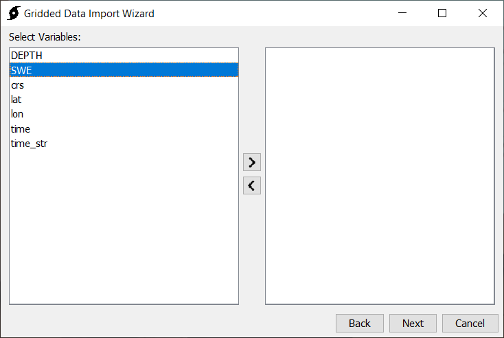
Click on SWE in the left hand list, as shown in the screenshot below, and press the right arrow to select SWE. It will now appear in the right-hand list.
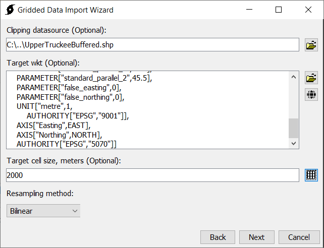
Click next and specify clipping extent, projection and resampling parameters in the dialog:
- Use the buffered project extent file UpperTruckeeBuffered.shp, provided in the ClippingExtent.zip folder in the Project Files section above.
- The target wkt is a coordinate reference system (CRS) in well-known text (WKT) format. Use the globe button to the right to select the standard hydrologic grid (SHG) CRS.
- The target cell size is the cell size of the resampled grids. Use the grid button to the right to select 2000 meters to match the discretization grids of the project model discretization.
- The resampling method is the method used to resample the grid. Select the Bilinear resampling method for continuous data.
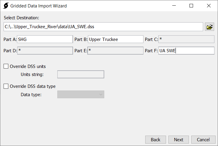
Click Next to select the destination HEC-DSS file. Browse to the project's data folder and create the new UA_SWE.dss file, as shown in the screenshot below. Enter A, B, and F parts which represent the grid type, geographic area, and data source, respectively. The C, D, and E parts will be auto-populated, based on the data. Note that the new clipped file is now less than 2 MB. Remove the original *.nc file out of the project data folder to decrease project size.
You can visualize the spatial SWE data for each time step by opening the UA_SWE.dss file with HEC-DssVue, selecting a record, and clicking on the Tabulate menu, as shown in the image below.
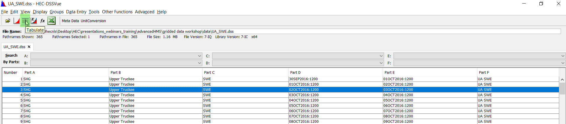
Note that some data is missing in the top right corner.

You can use the Vortex image-exporter utility to convert one of the records in the UA_SWE.dss file into *.tiff format to visualize whether the missing data will affect the project, and then use the Sanitizer tool (accessible through Tools | Data | Sanitizer menu, or as part of Vortex package) to explicitly address the missing data if necessary.
Add the imported SWE grid data to HEC-HMS model
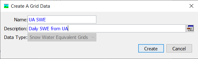
Create a new Snow Water Equivalent Grid from the Components | Grid Data Manager dialog.
Specify the grid name and provide a brief description.
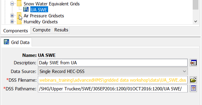
Now link the gridded SWE data in UA_SWE.dss file to the newly created UA SWE grid by clicking on the grid in the tree and selecting the DSS file name and pathway. Note that the DSS file name in the example below is highlighted yellow, because the file is outside of the project folder. It is recommended to save linked data files within the project folder to avoid losing them when transferring project files.
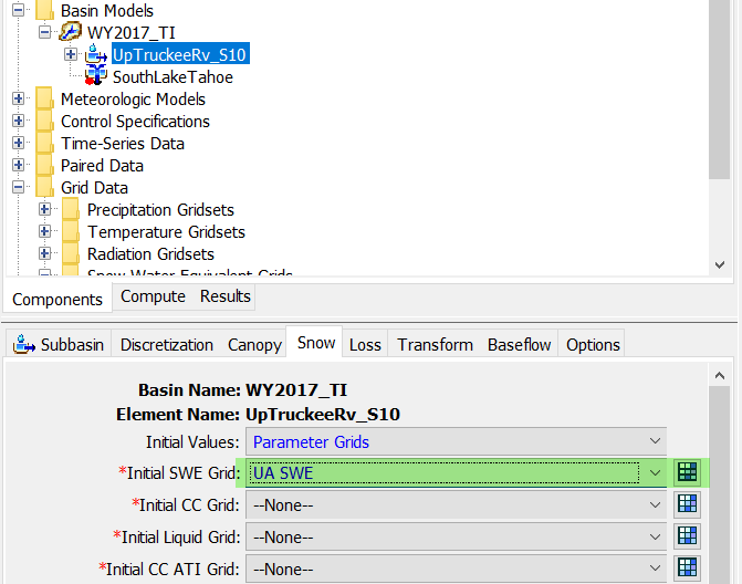
The UA SWE grid can now be used in the model, for example, it can be selected to specify initial SWE conditions for a subbasin snow method, as illustrated below. Change the snow method's Initial Values back to Default Values. You will instead use the SWE gridded data in Part 2 of this workshop to calculate subbasin-averaged SWE time series, which can be very helpful in calibrating a snowmelt model.
Importing temperature data
Download gridded PRISM temperature
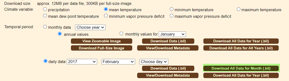
The PRISM climate group gathers climate observations from a wide range of monitoring networks and applies sophisticated quality control measures to develop gridded climate datasets. PRISM data is collected using a horizontal resolution of 800 meters and is provided to users at a resolution of 4 kilometers. Datasets are available in ASCII (“.asc”) or BIL (“.bil”) format. Data is available from 1981 to present for most PRISM products including 30-year normals, daily, and monthly records. Daily PRISM data was downloaded for this tutorial. More information about PRISM climate data can be found at the PRISM Climate Data website.
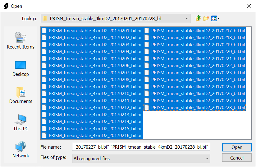
Data can be downloaded directly from the PRISM website under the “Recent Years” tab. For this workshop, download daily data for February 2017. Zipped data in *.bil format. It is also available in Project FIles section above.
Import temperature into HEC-DSS format
Open Gridded Data Importer and follow the steps outlined for the SWE data to select all daily temperature *.bil files.
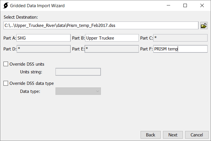
Clip, project and resample the files, as shown in the screenshot below. Use the buffered project extent file UpperTruckeeBuffered.shp, provided in the ClippingExtent.zip folder in the Project Files section above.
Finally, save the grids to a new Prism_temp_Feb2017.dss file in the project data folder.
Add temperature grid data to HEC-HMS model
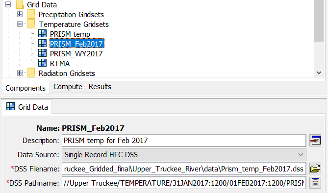
From the Components | Grid Data Manager dialog, create a new Temperature Gridset titled PRISM_Feb2017 and connect it with the gridded data in the Prism_temp_Feb2017.dss file.
Use temperature grid in a compute
You will now add the PRISM temperature grid that you just created to a meteorological model, and run a compute to compare the modeled SWE for February 2017 to the modeled SWE using another gridded temperature data source - hourly RTMA grid data. The Real-Time Mesoscale Analysis (RTMA) is a NOAA/NCEP high-spatial and temporal resolution analysis/assimilation system for near-surface weather conditions (NCEP). It produces hourly analyses at 1.25-3 km resolution.
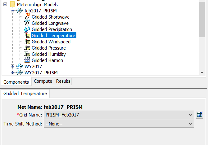
First, copy the WY2017 Met model and name the copy Feb2017_PRISM. Click on Gridded Temperature for the new met model in the project tree and change the referenced grid name from RTMA to PRISM_Feb2017.
Create two computes:
| Name | Feb2017_TI_RTMA |
|---|---|
| Basin | WY2017_TI |
| Meteorologic Model | WY2017 |
| Control Specification | Feb2017 |
| Name | Feb2017_TI_PRISM |
|---|---|
| Basin | WY2017_TI |
| Meteorologic Model | Feb2017_PRISM |
| Control Specification | Feb2017 |
The WY2017_TI basin models snowmelt with the Gridded Temperature Index method, which uses air temperature as a proxy for the energy available for heating or melting the snowpack. Run both models and examine results. To display both of the modeled SWE and the observed SWE graphs on one chart, Ctrl+click to select the corresponding time-series in the tree, and then click on the Graph icon, as shown in the figure below.
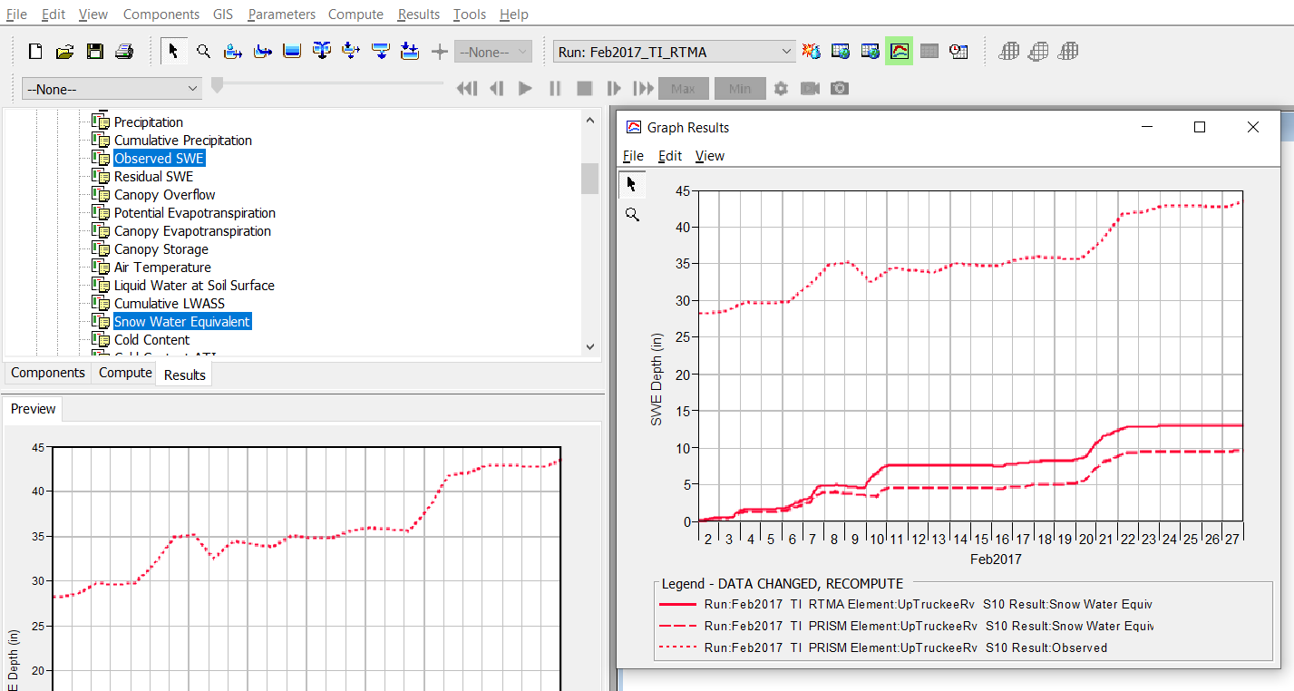
The resulting modeled SWE for February 2017 is different with the two temperature data sources, as can be seen in the figure below. The results should not be directly compared to the observed SWE, because the compute was started with zero initial conditions.
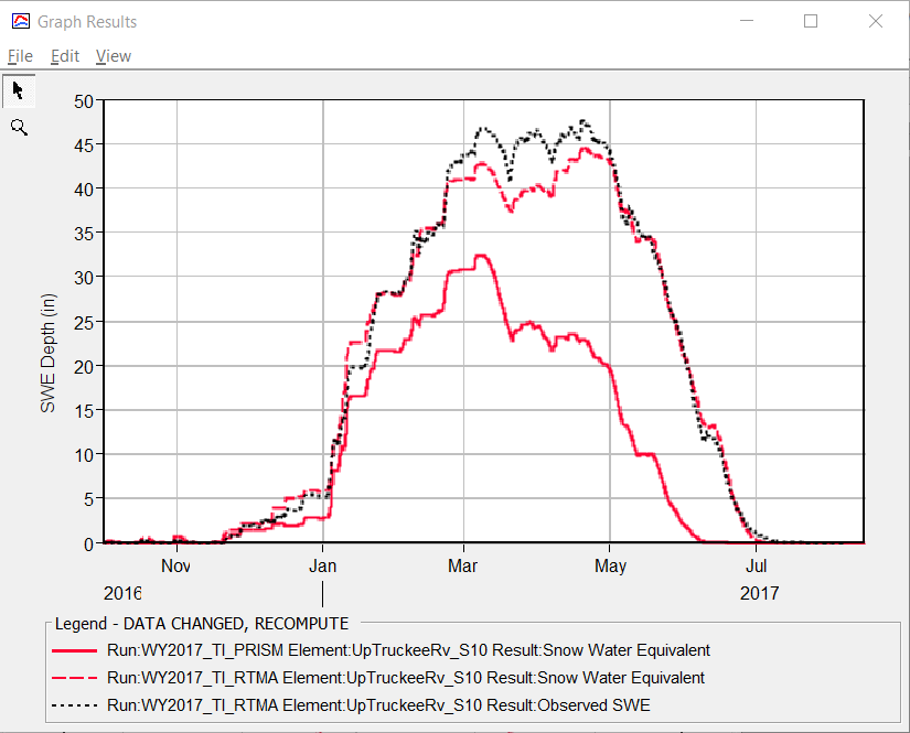
A new meteorological model and compute with the PRISM gridded temperature data sources for the entire WY2017 (WY2017_PRISM) was created for you in the model. The figure below compares the modeled and observed SWE with the RTMA and PRISM gridded temperature sources for WY2017.
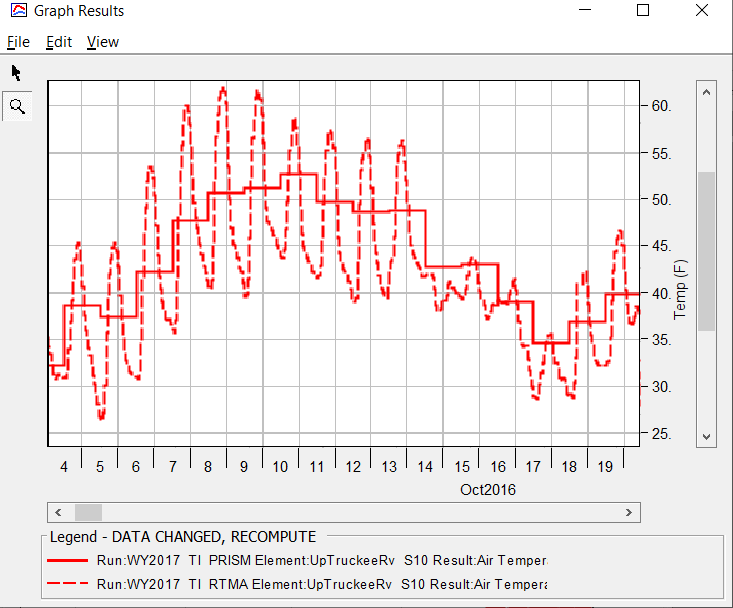
Discussion Question 1: What could be some of the causes for the difference in modeled SWE between the two temperature sources?
One reason could be the difference in time step: RTMA is hourly and PRISM is daily. Daily average temperature does not adequately capture the daily extremes.
Discussion Question 2: Do you expect the results to change if the PRISM temperature data was resampled at smaller cell size?
No, because PRISM temperature data is at 4km resolution.
Discussion Question 3: Could anything be done to make the modeled SWE better fit the observed data using PRISM temperature?
The model was calibrated to the hourly RTMA temperature. Recalibrating the model with the daily PRISM input could potentially improve the fit.
Optional: visualize gridded temperature results
HEC-HMS allows the user to visualize gridded result, provided that subbasin elements are georeferenced. Spatial results will be displayed at the discretization level for the subbasin elements. If you have time, go through the steps in the Spatial Results Tutorials to visualized gridded air temperature for the subbasin. Hint: you will need to rerun the computes with the Spatial Results option selected.
Project Files
Continue to: Part 2a: Creating Area-Averaged Time Series with HEC-HMS Grid to Point Tool.
Return to: Workflows for Downloading, Importing and Manipulating Gridded Data.