Last Modified: 2024-05-17 08:48:18.919
This workshop can be completed as part of the Workflows for Downloading, Importing and Manipulating Gridded Data or as a stand-alone activity.
HEC-HMS version 4.11-beta.10 was used to create this example. You can open the example project with HEC-HMS v4.11 or a newer version.
 UA_SWE.dss
In the Introduction to Gridded Snowmelt Calibration workshop, subbasin-average SWE computed by HEC-HMS was compared against output from the National Operational Hydrologic Remote Sensing Center (NOHRSC) Snow Data Assimilation System (SNODAS). You will now use the Grid To Point tool in HEC-HMS to create a subbasin-averaged observed SWE time series from the University of Arizona gridded snow water equivalent (UA SWE) data that you created in Task 1: Importing Gridded Data and compare it to the time series derived from the SNODAS SWE data.
To start, download the initial project files for the Upper Truckee River watershed above, or use your project from Part 1. Browse to the project's data folder. If the folder doesn't already have the UA_SWE.dss file, you can upload a copy from the Project Files section above.
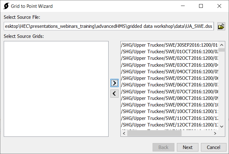
Open the Upper Truckee River project. Go to Tools | Data | Grid To Point to open the wizard. Browse to the UA_SWE.dss file, highlight all source grids on the left-hand side (Ctrl + A) and click the right arrow to select them. The wizard dialog should match the figure below.
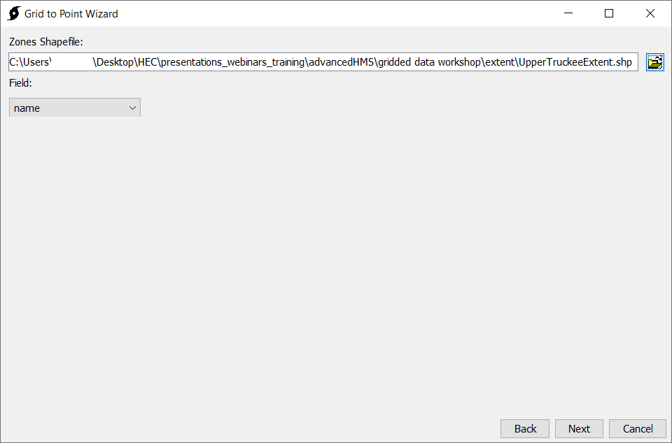
In the next dialog, select the Zones Shapefile to indicate the region over which the gridded data will be averaged. Use the Clipping Extent shapefile from Part 1 of this workshop (or download form Project Files if needed).
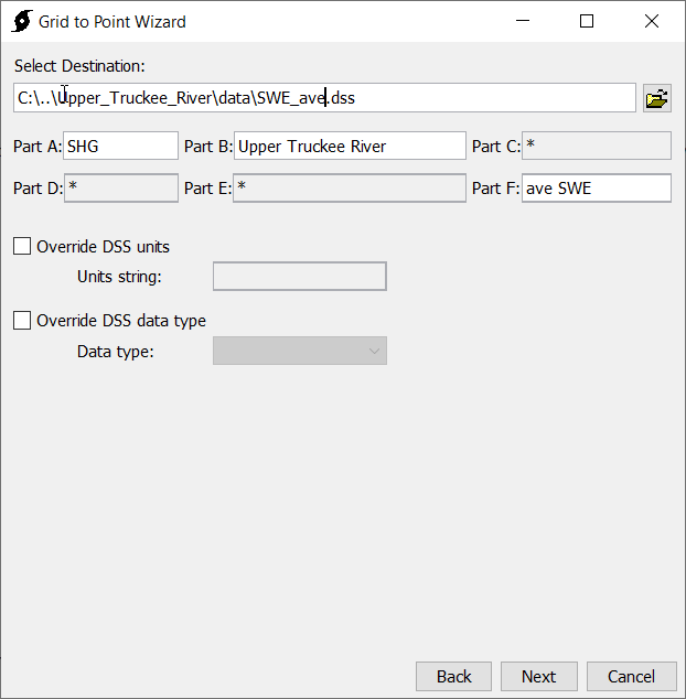
Name the output file SWE_ave.dss and save in the project's data folder.
Create a new snow water equivalent gage named UA SWE Gage from the Time Series Data Manager.

Browse to the new UA SWE Gage in the project tree and link it to the SWE_ave.dss file.
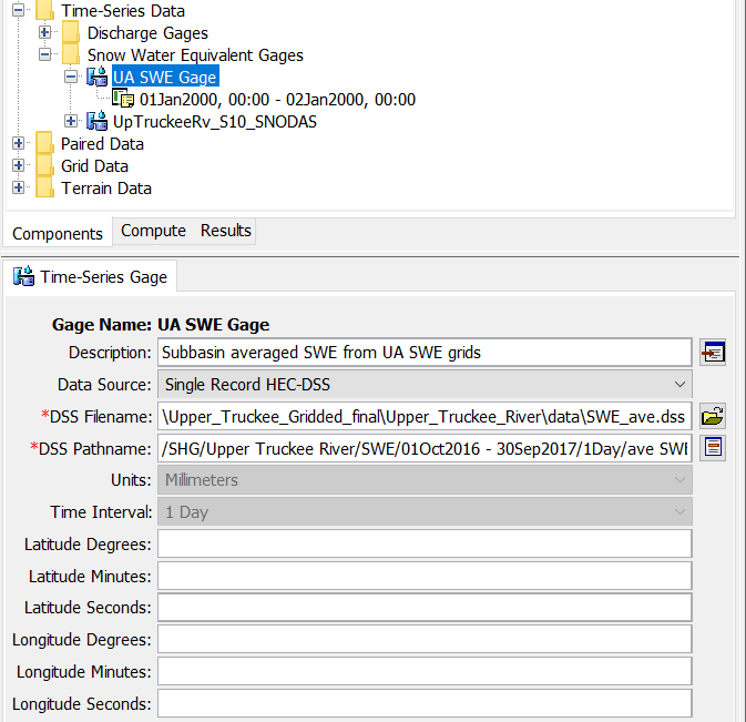
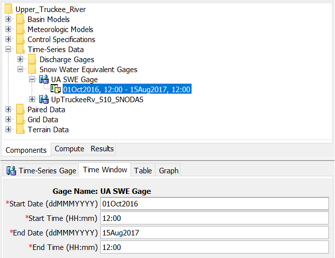
Click on time window in the tree and change it to match the available data, as shown in the image below. You can now visualize the average time series by clicking on the Graph tab.
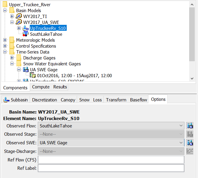
Now link the time series gage to the observed SWE for a subbasin. Create a copy of the WY2017_TI basin model and name it WY2017_UA_SWE. Click on the UpTruckeeRv_S10 subbasin's Options tab and switch observed SWE gage to the new UA SWE Gage.
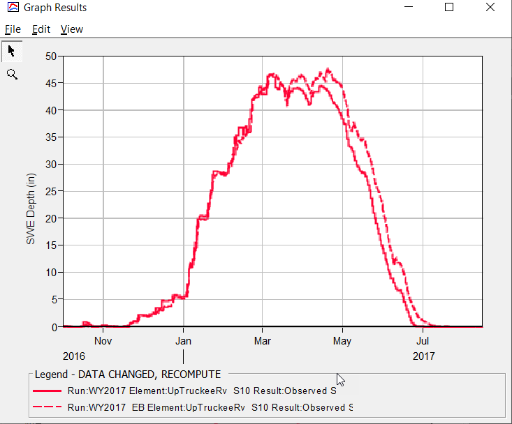
Create a new WY2017_TI_US_SWE compute and link it to the WY2017_UA_SWE basin model, the WY2017 meteorologic model, and the WY2017 control specifications. Run both the new compute and the existing WY2017_TI_RTMA compute. Compare the results by plotting the observed SWE for the two models. The solid line is the averaged UA SWE data and the dotted line is the averaged time series of the SNODAS SWE. The similarity between the two sources provides a quality check on the gridded data.
Continue to: Part 2b: Selecting a Normalization Interval.
Return to: Workflows for Downloading, Importing and Manipulating Gridded Data.