Download PDF
Download page Optimizing Gridded Precipitation.
Optimizing Gridded Precipitation
Last Modified: 2024-09-05 10:57:36.071
Project Version
HEC-HMS version 4.12 was used to create this tutorial. You will need to use HEC-HMS version 4.12, or newer, to open the project files.

Introduction
In the previous tutorial, Transposing Gridded Precipitation, you calculated storm depths, transposed the precipitation, and applied a bias grid to the observed gridded precipitation data. When comparing the results from the different simulation runs, peak flows varied at the point of interest, Mahoning Creek Gage at Punx. Assuming that your goal is to maximize peak flows at the downstream gage, the results demonstrated that simply moving the storm center to a point closer to the watershed is not a reliable way to increase peak flows. The user could continue an iterative process of selecting new storm center coordinates within the transposed meteorologic model until the desired result is achieved. HEC-HMS can automate this process. In this tutorial, you will use the Optimization tools in HEC-HMS to automatically select a storm center location that maximizes peak flows at the point of interest. You will pick up where the Transposing Gridded Precipitation tutorial left off. Download and unzip the Optimizing_Gridded_Precipitation_Initial.zip file.
Task 1: Set up the Optimization Trial
- Select Compute | Optimization Trial Manager and create a new Optimization Trial named Maximum Peak Flow. Select Sep2018 as the Basin Model and Sep2018_transposed as the Meteorologic Model.
- Go to the Compute tab and select the new Optimization Trial to open the Optimization Trial Editor.
- Check that Sep2018 selected as the Basin Model and Sep2018_transposed as the Meteorologic Model.
- Set the time window to 01Sep2018 0000 to 16Sep2018 0000. This captures the precipitation event driving peak flows as well as the rise and fall of the hydrograph. If you were to shorten the time window to start closer to the major precipitation, you would simply need to adjust the initial losses because this model was calibrated for an event beginning 01Sep2018. The Optimization Trial Editor should look like the figure below.

Task 2: Define the Search Parameters and Set Objective
- Go to the Search tab and Select Simplex as the Method. Set Max Iterations to 100 and Tolerance to 0.01. Leave the Tolerance Criteria as the default Absolute. The Search Editor should look like the top figure below.
- Go to the Objective tab and Select Maximiazation as the Goal. Set Location to Mahoning Creek Gage at Punx. Select Discharge as the Time-Series. Select Peak Discharge as the Statistic. Select No Transform for the Data Transformation. The Objective Editor should look like the bottom figure below.


Task 3: Add Gridded Precipitation Parameters
- Right-click on the Optimization Trial name in the Watershed Explorer and Select Add Parameter. Click on the new Parameter 1 to open the Optimization Parameter Editor.
- Select Precipitation Parameters as the Element. Double-click Gridded Precipitation X-Coordinate in the Parameter dropdown. This will fill in the initial value of the X-coordinate set in the Sep2018_transposed Meteorologic Model. Leave Locked dropdown set to No.
- The default bounds for the parameter are very wide. The limits should be set to more realistic values so that the optimization will converge within a reasonable number of iterations. For the X-coordinate parameter, input bounds of 4,493,600 ft to 4,820,600 ft. These bounds were chosen based on the extent of the input gridded dataset.
- Repeat Steps 8 and 9 for the Gridded Precipitation Y-Coordinate parameter. For the Y-coordinate parameter, input bounds of 6,822,400 ft to 7,052,000 ft. These bounds were chosen based on the extent of the input gridded dataset. You should now have two parameters in this Optimization Trial.


Task 4: View and Interpret the Results
- Run the Maximum Peak Flow Optimization Trial and view Summary Results at Mahoning Creek Gage at Punx. The optimized peak flow is 11,339 cfs.
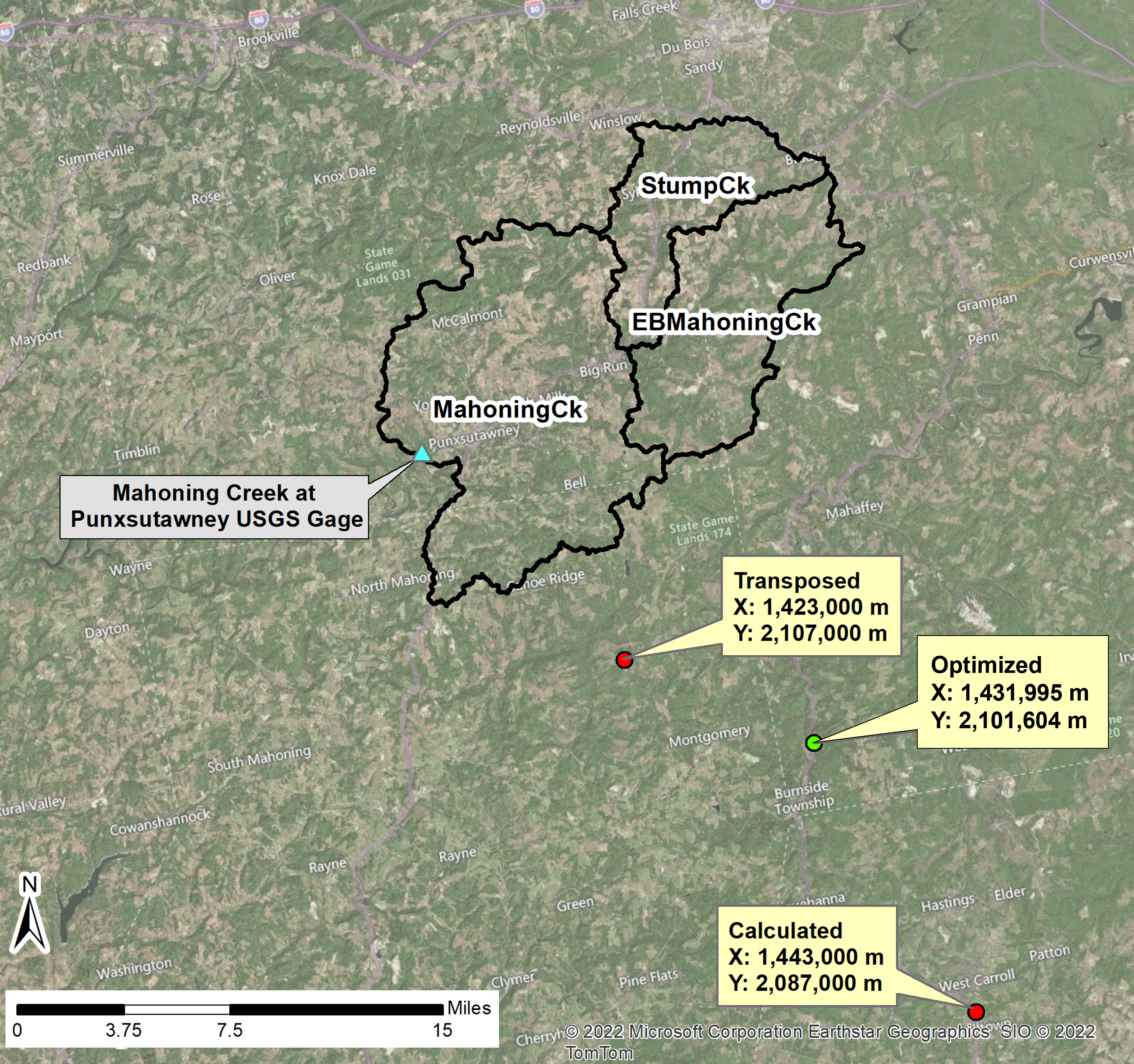
- Select the Optimized Paramters results table to view the optimized storm center coordinates. Overall, the original calculated storm center of X: 4,733,040 ft Y: 6,845,360 ft was shifted 34,895 ft west and 49,666 ft north to an optimized center of X: 4,698,145 ft Y: 6,895,026 ft (X: 1,431,995 m Y: 2,101,604 m).
- Select the Objective Function graph to view how the Optimization Trial converged and the number of evaluations within the final iteration. This trial completed in 34 iterations total.


You can compare the optimized peak flow result and optimized storm center coordinates to the peak flow results and storm center coordinates from the Transposing Gridded Precipitation tutorial. The optimized storm center increased the peak flow at the downstream gage by approximately 2,700 cfs over the observed gridded precipitation data. The map shows that the optimized storm center has shifted closer to the watershed, but is not within the watershed's bounds. It's important to note that while the transposed storm center is closer to the watershed, the optimized storm center yields higher peak flows.
| Simulation | Peak Flow, cfs |
|---|---|
| Sep2018_observed | 8,637 |
| Sep2018_transposed | 10,400 |
| Sep2018_transposed_biased | 10,123 |
| Optimization Trial: Maximum_Peak_Flow | 11,339 |
Task 5: View Spatial Results
You now have the optimized storm centers generated in Task 4 and can create a transposed storm center meteorologic model and simulation run to view spatial results for this optimized storm center.
- Input the optimized coordinates into the Sep_2018_optimized meteorologic model and Run the Sep2018_optimized simulation run.
- Select the Sep2018 Basin Model so that the subbasins display in the Watershed Explorer. Select Sep2018_optimized in the Computation Selection dropdown.
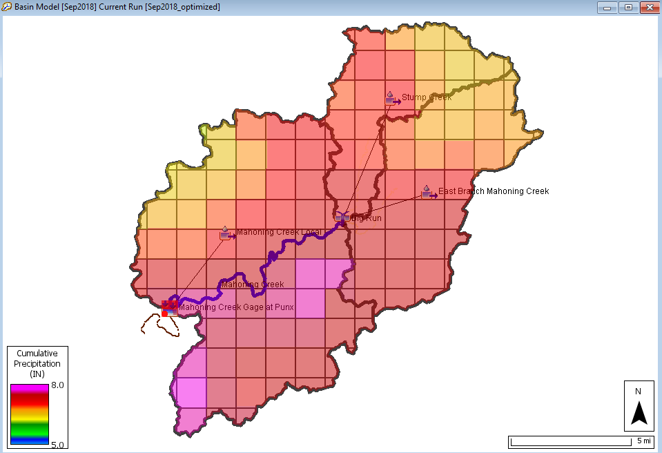
- Select Cumulative Precipitation in the Spatial Results toolbar dropdown. Click Max to view the max cumulative precipitation results.
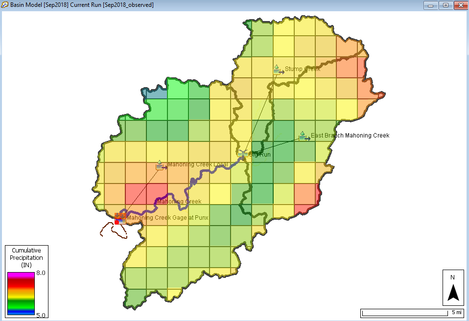
- Repeat steps 1 and 2 for Sep2018_observed. Spatial results display settings can be adjusted by selecting the gear icon in the Spatial Results toolbar. Setting the same Minimum and Maximum values and Color Scheme can help simplify the visual comparison of the two simulations.
- Compare Sep2018_optimized to Sep2018_observed Spatial Results. You can hover over a subbasin to see the Maximum Cumulative Precipitation within that cell.
The Sep2018_observed spatial results (below) show the distribution of cumulative precipitation based on the observed dataset's calculated storm center.
The Sep2018_optimized spatial results (below) show the distribution of cumulative precipitation based on the optimized storm center location. Compared to the observed dataset , there is an increase in accumulated precipitation throughout the watershed.