Download PDF
Download page Transposing Gridded Precipitation.
Transposing Gridded Precipitation
Last Modified: 2024-09-05 10:58:22.964
Project Version
HEC-HMS version 4.12 was used to create this tutorial. You will need to use HEC-HMS version 4.12, or newer, to open the project files.

Introduction
In this tutorial, you will use storm centering functionality available with a gridded precipitation method in an HEC-HMS meteorological model to calculate the area of maximum rainfall and shift or transpose the precipitation to a different part of the watershed. The ability to shift a storm from one area to another nearby area with similar meteorologic characteristics allows the user to apply precipitation data to desired locations with missing or unavailable records based on spatial proximity. This is known as a substituting space for time. Find more information on working with and obtaining Gridded Precipitation data in the Gridded Precipitation Method Tutorial and Gridded Data Sources Guide.
You will be working with the Punxsutawney Watershed. The Punxsutawney Watershed (154 sq. mi) is part of the Allegheny River Basin located in western Pennsylvania, USA. In this tutorial, you will work through the following tasks to analyze and manipulate observed gridded precipitation data: 1) Calculating the storm center 2) Transposing the storm center and 3) Applying a bias correction to gridded precipitation. Download and unzip the Transposing_Gridded_Precipitation_Initial.zip file.

Task 1: Import Gridded Precipitation in Gridded Precipitation Editor
Gridded precipiation data for the September 2018 storm event has been downloaded and saved within the project directory. You will need to create a gridded dataset and import the associated DSS record for the September 2018 event.
- Select Components | Grid Data Manager to open the Grid Data Manager Dialog. In the Grid Data Dialog, Select Precipitation Gridsets from the Data Type dropdown.
- Click New and name the dataset QPE. Close the Grid Data Manager dialog.
- In the Watershed Explorer, expand the Grid Data folder and the Precipitation Gridsets folder. Select the QPE Gridded Dataset that you just created.
- Select Single Record HEC-DSS in the Data Source dropdown. Click on the file chooser icon and navigate to the Data Folder in your project directory and Select precip.dss. Select the path chooser icon and Select the first record: ///PRECIPITATION/31AUG2018:2300/31AUG2018:2400//.
- Save the project to commit your DSS file and path selections.

Task 2: Calculate the Storm Center
You may have noted that Calculate Storm Centers Buttons are disabled until a Single Record HEC-DSS file and pathname are chosen in the Gridded Precipitation Editor. This is because when the storm center is calculated by the HEC-HMS model, it is accumulating precipitation at each grid cell from the first timestep to the last time step. Each record in the DSS file represents a time step. The calculated storm center is the location of the grid cell with the maximum precipitation depth.
- Click the X-coordinate Calculator Button to compute the easting coordinate of the September 2018 storm center.
Click the Y-coordinate Calculator Button to compute the easting coordinate of the September 2018 storm center.
Make note of the calculated coordinates. X-coordinate: 1,443,000 meters Y-coordinate: 2,087,000 meters.
- In the Watershed Explorer, expand the Meteorologic Models and select Gridded Precipitation under Sep 2018_observed Meteorologic Model to open the Meteorologic Model Component Editor.
- In the Grid Name dropdown, Select QPE. Leave the Time Shift option set to None.
Run the Sep2018_observed simulation from the toolbar ribbon or by right-clicking on the simulation in the Compute tab and clicking Compute.


Coordinate System
The X-coordinate and Y-coordinate will be calculated and displayed in units of the DSS grid file. These units can be verified by opening the grid in HEC-DSSVue.To verify the coordinate system of your precipitation grid, open the precip.dss file in HEC-DSSVue. Right-click on any record and Select Edit. Within the dialog box, Select Detailed Grid Info tab to see the important metadata about the grid including the Data Units, Cell Size, Grid Coordinate System, and Grid Projection Units. From the dialog we can see that this grid contains precipitation depths in units of millimeters and a cell size of 2000 meters. The projected coordinate system is Albers NAD83 meters.
Task 3: Apply a Transpose in Meteorologic Model
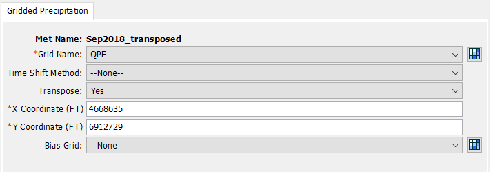
- In the Watershed Explorer, expand the Meteorologic Models and select Gridded Precipitation under Sep 2018_transposed Meteorologic Model to open the Meteorologic Model Component Editor.
- In the Grid Name dropdown, Select QPE. Leave the Time Shift option set to 0.
- Select "Yes" in the Transpose dropdown. New inputs fields will appear for an X-coordinate and Y-coordinate. A Bias Grid dropdown menu will also appear, leave this field set to None for now.
- The X-coordinate and Y-coordinate fields for the Transpose option must be input as absolute units. For this example, let's assume we want to shift the storm center a 20,000 meters (65,617 feet) to the west and 20,000 meters (65,616 feet) to the north so that the storm center is closer to the watershed. Remember, the X-coordinate is positive in the east direction and the Y-coordinate is positive in the north direction. While the storm coordinates computed in Task 2 are shown in meters to match the unit system of the precipitation grid, the transposition coordinates will be input in absolute units of the model. In this case, the model units are feet and the coordinates of the computed storm center in feet are X-coordinate: 4,734,252 feet Y-coordinate: 6,847,113 feet. To perform the shift, input 4668635 for the new X-coordinate and 6912730 for the Y-coordinate. Do not use comma separators when inputting coordinates.
- Run the Sep2018_transposed Simulation. In the Message Log, see that NOTE 20143: Storm shift X: -65616.798 ft, Y: 65616.798 ft. is displaying the storm shift relative to the storm centers calculated in Task 2. If you don't see this message displayed within the message log, you can check the Sep2018_transposed.log file in the project's directory for the full list of messages from the simulation run.
The map shows the location of the calculated storm center and the transposed storm center in relation to the Punsutawney subbasins and downstream streamgage.
![]()
Task 4: Import a Precipitation-Normal Grid
- Select Components | Grid Data Manager to open the Grid Data Manager dialog. Select Precipitation-Normal Grids and Click New.
- Name the new Grid Dataset NOAA24HR_100YR.
- Navigate to Precipitation-Normal Grids under Grid Data in the Watershed Explorer. Open the NOAA24HR_100YR under the Precipitation Gridsets.
- On the Grid Data Editor the Select GeoTIFF as the Data Source.
- Click the File chooser button and navigate to the \Transposing_Gridded_Precipitation_Initial\Punx_HMS\gis folder in the project directory. Select the NOAA_24HR_100YR.tif.
- Set the units to in for inches and the Unit Scale Factor to 1000.

Task 5: Apply a Bias Correction in Meteorologic Model
A Bias Correction can be applied to transposed gridded precipitation when the user wants to adjust, or pattern, the distribution of precipitation in the gridded dataset. It is typically used when a watershed includes mountainous regions where terrain plays a significant role in the magnitude of precipitation. The bias will be applied to the grid based on relative depths of the observed bias grid about the calculated storm center as compared to the transposed storm center. The NOAA 24-hr 100-year precipitation grid will be used as the bias grid. The biasing computation is detailed in Bias Adjustment For Transposed Precipitation guide.
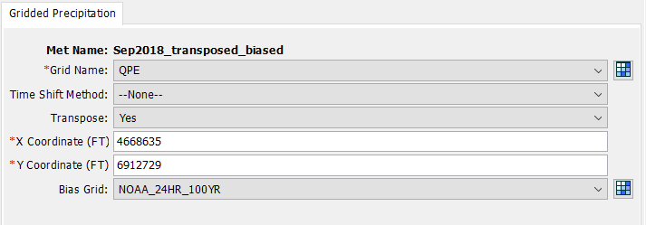
- Select Sep2018_transposed_biased Meterorologic Model to open the Meteorologic Model Component Editor.
- Select "Yes" in the Transpose dropdown. Input 4668635 for the new X-coordinate and 6912729 for the Y-coordinate. Do not use comma separators when inputting coordinates.
- Select the NOAA_24HR Precipitation-Normal Grid in the Bias Grid dropdown.
- Run the Sep2018_transposed_biased Simulation.
Task 6: Compare Peak Flow and View Spatial Results
View the global summary at the downstream gage Mahoning Creek Gage at Punx for each of the three simulation runs. Compare and analyze the peak flow results: The transposition of the storm center leads to an increase of peak flow at the downstream gage. The biasing of the transposed storm leads to a slight decrease in peak flow in comparison with the unbiased transposed storm. This is due to the comparison of precipitation depths within the bias grid.
| Simulation | Peak Flow, cfs |
|---|---|
| Sep2018_observed | 8,637 |
| Sep2018_transposed | 10,407 |
| Sep2018_transposed_biased | 10,123 |
You can also compare Spatial Results of Cumulative Precipitation to better visualize how shifting storm center location impacts precipitation depths over the subbasins. For additional guidance on configuring your model for Spatial Results, refer to the Viewing Spatial Results tutorial.
- Select the Sep2018 Basin Model so that the subbasins display in the Watershed Explorer. Select Sep2018_observed in the Computation Selection dropdown.
- Select Cumulative Precipitation in the Spatial Results toolbar dropdown. Click Max to view the max cumulative precipitation results.
- Repeat steps 1 and 2 for Sep2018_transposed and Sep2018_transposed_biased. Spatial results display settings can be adjusted by selecting the gear icon in the Spatial Results toolbar. Setting the same Minimum and Maximum values and Color Scheme can help simplify the visual comparison of the two simulations.
- Compare Sep2018_observed to Sep2018_transposed and Sep2018_transposed_biased Spatial Results. You can hover over a subbasin to see the Maximum Cumulative Precipitation within that cell.
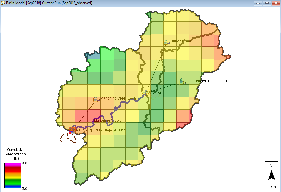
The Sep2018_observed spatial results (below) show the distribution of cumulative precipitation based on the observed dataset's calculated storm center.
The Sep2018_tranposed spatial results (below) show the distribution of cumulative precipitation based on your selected transposed location. Compared to the observed dataset, more precipitation accumulated throughout the watershed.
![]()
The Sep2018_tranposed_biased spatial results (below) show the distribution of cumulative precipitation based on your selected transposed location with a bias grid added. As expected, the pattern of precipitation depths matches the transposed unbiased case but the magnitude is slightly decreased based on the NOAA 24 HR 100 YR precipitation depths. Hover over individual cells in the biased and unbiased results plot to see the slight change in total precipitation with the bias grid added.
![]()
The comparison of spatial results for all three scenarios shows the increase in cumulative precipitation within the subbasins after transposition of the storm center leading to an increase in peak flows at the downstream gage and a slight decrease when a bias adjustment is applied. Suppose the desired goal of transposition was to find the storm center location that leads to the maximum peak flow at the downstream gage. The Optimizing Gridded Preicipitation tutorial will show you how HEC-HMS can be used to automate the transposition of the storm center based on the user's goal.