Applying the Save States Option to Support Changing Land Use Conditions

Introduction

Click HERE to access a tutorial that shows an example using the save and start states tool to initialize gridded snowmelt states within a forecast alternative simulation. Save and start states can also be applied in a regular simulation run. This tutorial shows how the save and start states tool can be used to transfer the soil moisture state from one simulation to another.

HEC-HMS version 4.9 beta 6 was used to create this tutorial.

You can download a copy of the dataset here – Russian_River_final.zip.

Modelers have requested options to change model parameters during a simulation, this option is commonly referred to as time variable parameters. There are a few examples where some HEC-HMS parameters can be set to vary throughout a year. The HEC-HMS team is planning to add a general framework that allows modelers to vary parameters either within a year, or throughout time. One common application of time variable parameters is modeling changes in percent impervious area as land use change occurs. Urbanization in a watershed can increase runoff magnitude and volume because precipitation is no longer able to infiltrate into the soil.

HEC-HMS contains options for modeling single events and long term simulation. Long term simulation requires additional hydrologic processes, like evapotranspiration, canopy storage, and baseflow, which are included in HEC-HMS. An HEC-HMS simulation could be configured to run a 60-year period at a 1-hour time step. However, changes to the percent impervious area, or the addition of storage structures would require modelers to break the 60-year period up into shorter time windows and use basin models with the appropriate configuration and parameterization. The save and start states option can be used to transfer model states, like the soil moisture state, from one simulation to another. When using save and start states in this way, the continuous simulation is a series of simulations (with shorter time windows), but states are being transferred from one simulation to the next.

Example

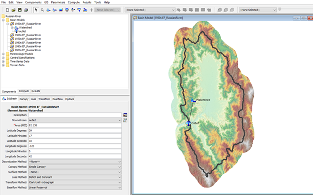
The example used here is loosely based on an actual watershed and data. The main point of the tutorial is to illustrate an application of save and start states; therefore, model calibration and validation are not included. A watershed in California is used for this example. As shown in the figure below, the 92 square mile watershed was represented with one subbasin element. The simple canopy, deficit and constant loss, Clark unit hydrograph transform, and linear reservoir baseflow methods were used. Subbasin average precipitation and evapotranspiration were specified in the meteorologic model. Precipitation and temperature data were available from January 1, 1950 through December 31, 2009.

You will notice in the figure below, and in the project, that there are six basin models. Each basin model contains a different percent impervious area parameter. For the sake of the tutorial, the percent impervious values represent the state of the watershed for approximately 10 years. The impervious area was set to 0% for the subbasin in the 1950s EF_RussianRiver basin model (represents a pre-developed watershed). The impervious area was increased to 5% in the 1960s basin model, 10% in the 1970s basin model, 15% in the 1980s basin model, 25% in the 1990s basin model, and 50% in the 2000s basin model.

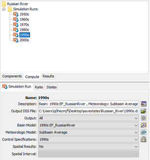
One single 60-year simulation would not capture changes to the percent impervious area in the watershed. As shown below, six individual simulations were configured. As an example, the 1990s simulation used the 1990 EF_RussianRiver basin model, the Subbasin Average meteorologic model, and the 1990s control specifications.

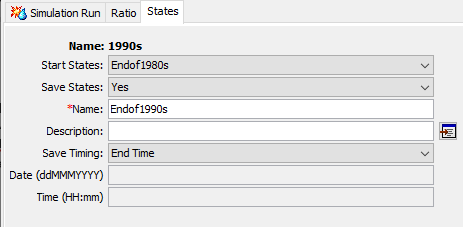
Initial conditions become an issue when breaking up a 60-year simulation into six decade long simulations. The start and save states option was used to transfer the states at the end of one simulation to the beginning of the next simulation. The figure below shows the States tab for the 1990s simulation. Notice the states saved at the end of the 1980s simulation is selected (named Endof1980s), and then the 1990s simulation was configured to write out final state variables at the end of the simulation. The Endof1990s state variables were used to initialize the 2000s simulation.

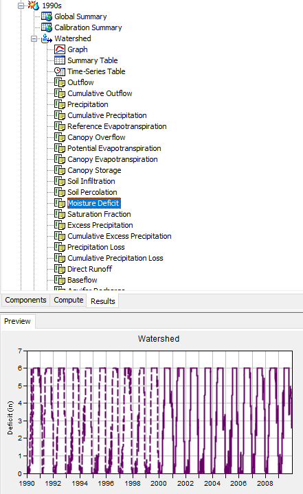
Once configured correctly, the six simulations were run in chronological order to effectively create results that reflect one long 60-year simulation where the percent impervious area was updated for each decade. The figure below shows the Results tab in the Watershed Explorer. The Moisture Deficit time-series was selected for both the 1990s and 2000s simulations. Hold down the control key to add multiple results to the same plot.

The following figure was created by pressing the View Graph for Selected Element(s) button. The plot properties were edited to use different colors for both simulations. The zoom in option was used to show the transition in moisture deficit from the 1990s to 2000s simulations. Notice the 2000s simulation was initialized using the final moisture deficit from the 1990s simulation.

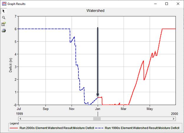
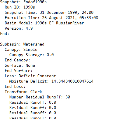
The following figure shows a portion of the Endof1990s.state file located in the … \Russian_River\basinStates directory. The moisture deficit at the end of the 1990s simulation was 14.34 millimeters (0.565 inches). Until the HEC-HMS team releases new capability to define time variable parameters, the save and start states option is one way to configure a long term simulation where model parameters could be adjusted.