Kinematic Wave Transform Model

The kinematic wave method is a conceptual model of watershed response. This model represents a watershed as an open channel (a very wide, open channel), with inflow to the channel equal to the excess precipitation. Then it solves the equations that simulate unsteady shallow water flow in an open channel to compute the watershed runoff hydrograph. This model is referred to as the kinematic-wave model. Details of the kinematic-wave model implemented in the program are presented in HEC's Training document No. 10 (USACE, 1979).

Basic Concepts and Equations

The kinematic wave method utilizes simplifications of the open channel flow equations to route excess precipitation to the subbasin outlet. This approximation starts with a one-dimensional approximation of the momentum equation :

1)	$\begin{array}{l}\displaystyle S_f=S_0-\frac{\partial y}{\partial x}-\frac{V}{g} \frac{\partial V}{\partial x}-\frac{1}{g} \frac{\partial V}{\partial t}\end{array}$

where S_f = energy gradient (or friction slope) [ft/ft or m/m], S₀ = channel slope [ft/ft or m/m], V = velocity [ft/sec or m/sec], y = hydraulic depth [ft or m], x = distance along the flow path [ft or m], t = time [sec]; g = acceleration due to gravity [ft/sec² or m/sec²], ( $\begin{array}{l}\frac{\partial y}{\partial x}\end{array}$ ) = pressure gradient [ft/ft or m/m], (V/g)( $\begin{array}{l}\frac{\partial V}{\partial x}\end{array}$ ) = convective acceleration [ft/sec² or m/sec²], and (1/g)( $\begin{array}{l}\frac{\partial V}{\partial t}\end{array}$ ) = local acceleration [ft/sec² or m/sec²]. S_f can be approximated using Manning’s equation:

2)	$\begin{array}{l}\displaystyle Q=\frac{K}{N} R^{2 / 3} A \sqrt{S_f}\end{array}$

where K = 1.486 or 1.0 when using English units or metric units, respectively, Q = flow [ft³/sec or m³/sec], N = overland flow roughness coefficient, R = hydraulic radius [ft], and A = cross-sectional area [ft² or m²]. S_f can be set equal to S₀ when acceleration effects are negligible (i.e. steady, unvaried flow). Thus, Equation (2) can be simplified to:

3)	$\begin{array}{l}\displaystyle Q = \alpha A^m\end{array}$

where α and m = parameters related to flow geometry and surface roughness.

The one-dimensional continuity equation begins as :

4)	$\begin{array}{l}\displaystyle A \frac{\partial V}{\partial x}+V B \frac{\partial y}{\partial x}+B \frac{\partial y}{\partial t}=q\end{array}$

where B = top width [ft or m], A( $\begin{array}{l}\frac{\partial V}{\partial x}\end{array}$ ) = prism storage, VB( $\begin{array}{l}\frac{\partial y}{\partial x}\end{array}$ ) = wedge storage, B( $\begin{array}{l}\frac{\partial y}{\partial t}\end{array}$ ) = rate of rise, and q = lateral inflow per unit length [ft³/sec/ft or m³/sec/m]. Simplifying to shallow flow over a planar surface reduces Equation 4 to:

5)	$\begin{array}{l}\displaystyle \frac{\partial A}{\partial t}+\frac{\partial Q}{\partial x}=q\end{array}$

Combining Equation 3 with Equation 5 produces:

6)	$\begin{array}{l}\displaystyle \frac{\partial A}{\partial t}+\alpha m A^{m-1} \frac{\partial A}{\partial x}=q\end{array}$

Equation 6 represents the kinematic wave approximation of the equations of motion. HEC-HMS represents the overland flow component as a wide, rectangular channel of unit width such that m = 5/3, and:

7)	$\begin{array}{l}\displaystyle \alpha=K * \sqrt{S_f} * \frac{1}{N}\end{array}$

The kinematic wave method allows for the representation of variable scales of complexity within a watershed. A simple representation is shown in Figure below where one or two overland planes and a channel are included.

Simple Representation of a Watershed Using Kinematic Wave

A complex representation is shown in Figure below where overland planes, subcollectors, collectors, and a channel are included. For a detailed discussion of this method, the reader is directed to HEC (1993).

Complex Representation of a Watershed Using Kinematic Wave Reproduced from (Hydrologic Engineering Center, 1993)

Channel Flow Model

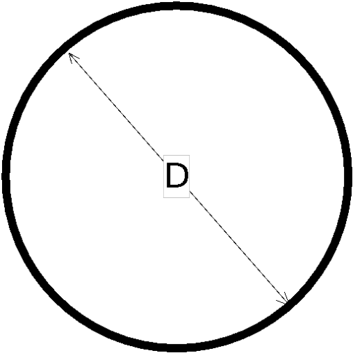
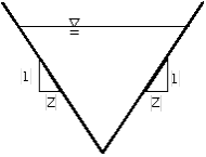
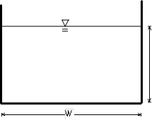
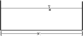
For certain classes of channel flow, conditions are such that the momentum equation can be simplified. In those cases, the kinematic-wave approximation of Equation 6 is an appropriate model of channel flow. In the case of channel flow, the inflow in Equation 6 may be the runoff from watershed planes or the inflow from upstream channels. Figure below shows values for $\begin{array}{l}\alpha\end{array}$ and m for various channel shapes used in the program.

The availability of a circular channel shape here does not imply that HEC-HMS can be used for analysis of pressure flow in a pipe system; it cannot. Note also that the circular channel shape only approximates the storage characteristics of a pipe or culvert. Because flow depths greater than the diameter of the circular channel shape can be computed with the kinematic-wave model, the user must verify that the results are appropriate.

Solution of Equations

The kinematic-wave approximation is solved in the same manner for either overland or channel flow:

The partial differential equation is approximated with a finite-difference scheme.
Initial and boundary conditions are assigned.
The resulting algebraic equations are solved to find unknown hydrograph ordinates.

The overland-flow plane initial condition sets A, the area in Equation 6, equal to zero, with no inflow at the upstream boundary of the plane. The initial and boundary conditions for the kinematic wave channel model are based on the upstream hydrograph. Boundary conditions, either precipitation excess or lateral inflows, are constant within a time step and uniformly distributed along the element.

Kinematic wave parameters for various channel shapes (USACE, 1998)

Circular Section

$\begin{array}{c}\alpha=\frac{0.804}{n} S^{\frac{1}{2}} D^{\frac{1}{6}} \\ m=5 / 4\end{array}$

Triangular Section

$\begin{array}{c}\alpha=\frac{0.94}{n} S^{\frac{1}{2}}\left(\frac{Z}{1+Z^{2}}\right)^{\frac{1}{3}} \\ m=4 / 3\end{array}$

Square Section

$\begin{array}{c}\alpha=\frac{0.72}{n} S^{\frac{1}{2}} \\ m=4 / 4\end{array}$

Rectangular Section

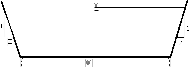
$\begin{array}{c}\alpha=\frac{1.49}{n} S^{\frac{1}{2}} W^{-\frac{2}{3}} \\ m=5 / 3\end{array}$

Trapezoidal Section

$\begin{array}{l}\displaystyle Q=\frac{1.49}{n} S^{\frac{1}{2}} A^{\frac{5}{3}}\left(\frac{1}{W+2 Y \sqrt{1+Z^{2}}}\right)^{\frac{2}{3}}\end{array}$

In Equation 6, A is the only dependent variable, as $\begin{array}{l}\alpha\end{array}$ and m are constants, so solution requires only finding values of A at different times and locations. To do so, the finite difference scheme approximates $\begin{array}{l}\partial A / \partial t\end{array}$ as $\begin{array}{l}\Delta A / \Delta t\end{array}$ , a difference in area in successive times, and it approximates $\begin{array}{l}\partial A / \partial x\end{array}$ as $\begin{array}{l}\Delta A / \Delta x\end{array}$ , a difference in area at adjacent locations, using a scheme proposed by Leclerc and Schaake (1973). The resulting algebraic equation is :

8)	$\begin{array}{l}\displaystyle \frac{A_{i}^{j}-A_{i}^{j-1}}{\Delta t}+\alpha m\left[\frac{A_{i}^{j-1}+A_{i-1}^{j-1}}{2}\right]^{m-1}\left[\frac{A_{i}^{j-1}-A_{i-1}^{j-1}}{\Delta x}\right]=\frac{q_{i}^{j}+q_{i}^{j-1}}{2}\end{array}$

Equation 8 is the so-called standard form of the finite-difference approximation. The indices of the approximation refer to positions on a space-time grid, as shown in Figure below. That grid provides a convenient way to visualize the manner in which the solution scheme solves for unknown values of A at various locations and times. The index i indicates the current location at which A is to be found along the length, L, of the channel or overland flow plane. The index j indicates the current time step of the solution scheme. Indices i-1, and j-1 indicate, respectively, positions and times removed a value $\begin{array}{l}\Delta x\end{array}$ and $\begin{array}{l}\Delta t\end{array}$ from the current location and time in the solution scheme.
Finite difference method space-time grid
With the solution scheme proposed, the only unknown value in Equation 8 is the current value at a given location, $\begin{array}{l}A_{i}^{j}\end{array}$ . All other values of A are known from either a solution of the equation at a previous location and time, or from an initial or boundary condition. The program solves for the unknown as :

9)	$\begin{array}{l}\displaystyle A_{i}^{j}=q_{a} \Delta t+A_{i}^{j-1}-\alpha m\left[\frac{\Delta t}{\Delta x}\right]\left[\frac{A_{i}^{j-1}+A_{i-1}^{j-1}}{2}\right]^{m-1}\left[A_{i}^{j-1}-A_{i-1}^{j-1}\right]\end{array}$

The flow is computed as :

10)	$\begin{array}{l}\displaystyle Q_{i}^{j}=\alpha\left[A_{i}^{j}\right]^{m}\end{array}$

This standard form of the finite difference equation is applied when the following stability factor, R, is less than 1.00 (see Alley and Smith, 1987):

11)	$\begin{array}{l}\displaystyle R=\frac{\alpha}{q_{a} \Delta x}\left[\left(q_{a} \Delta t+A_{i-1}^{j-1^{m}}\right)-A_{i-1}^{j-1^{m+}}\right] ; q_{a}>0\end{array}$

or

12)	$\begin{array}{l}\displaystyle R=\alpha m A_{i-1}^{j-1^{m-1}} \frac{\Delta t}{\Delta x} q_{a} ; \quad q_{a}=0\end{array}$

If R is greater than 1.00, then the following finite difference approximation is used:

13)	$\begin{array}{l}\displaystyle \frac{Q_{i}^{j}-Q_{i-1}^{j}}{\Delta x}+\frac{A_{i-1}^{j}-A_{i-1}^{j-1}}{\Delta t}=q_{a}\end{array}$

where is the only unknown. This is referred to as the conservation form. Solving for the unknown yields:

14)	$\begin{array}{l}\displaystyle Q_{i}^{j}=Q_{i-1}^{j}+q \Delta x-\frac{\Delta x}{\Delta t}\left[A_{i-1}^{j}-A_{i-1}^{j-1}\right]\end{array}$

When is found, the area is computed as

15)	$\begin{array}{l}\displaystyle A_{i}^{j}=\left[\frac{Q_{i}^{j}}{\alpha}\right]^{\frac{1}{m}}\end{array}$

Accuracy and Stability

HEC-HMS uses a finite difference scheme that ensures accuracy and stability. Accuracy refers to the ability of the solution procedure to reproduce the terms of the differential equation without introducing minor errors that affect the solution. For example, if the solution approximates $\begin{array}{l}\partial A / \partial x\end{array}$ as $\begin{array}{l}\Delta A / \Delta x\end{array}$ , and a very large $\begin{array}{l}\Delta x\end{array}$ is selected, then the solution will not be accurate. Using a large $\begin{array}{l}\Delta x\end{array}$ introduces significant errors in the approximation of the partial derivative. Stability refers to the ability of the solution scheme to control errors, particularly numerical errors that lead to a worthless solution. For example, if by selecting a very small $\begin{array}{l}\Delta x\end{array}$ , an instability may be introduced. With small $\begin{array}{l}\Delta x\end{array}$ , many computations are required to simulate a long channel reach or overland flow plan. Each computation on a digital computer inherently is subject to some round-off error. The round-off error accumulates with the recursive solution scheme used by the program, so in the end, the accumulated error may be so great that a solution is not found.
An accurate solution can be found with a stable algorithm when $\begin{array}{l}\Delta x / \Delta t \approx c\end{array}$ , where c = average kinematic-wave speed over a distance increment $\begin{array}{l}\Delta x\end{array}$ . But the kinematic-wave speed is a function of flow depth, so it varies with time and location. The program must select $\begin{array}{l}\Delta x\end{array}$ and $\begin{array}{l}\Delta t\end{array}$ to account for this. To do so, it initially selects $\begin{array}{l}\Delta x\end{array}$ = $\begin{array}{l}c\Delta t_m\end{array}$ where c = estimated maximum wave speed, depending on the lateral and upstream inflows; and $\begin{array}{l}\Delta t_m\end{array}$ = time step equal to the minimum of:

One-third the plane or reach length divided by the wave speed.
One-sixth the upstream hydrograph rise time for a channel.
The specified computation interval.

Finally, $\begin{array}{l}\Delta x\end{array}$ is chosen as: the minimum of this computed $\begin{array}{l}\Delta x\end{array}$ and the reach, or plane length divided by the number of distance steps (segments) specified in the input form for the kinematic-wave models. The minimum default value is two segments.
When $\begin{array}{l}\Delta x\end{array}$ is set, the finite difference scheme varies $\begin{array}{l}\Delta t\end{array}$ when solving Equation 61 or Equation 66 to maintain the desired relationship between $\begin{array}{l}\Delta x\end{array}$ , $\begin{array}{l}\Delta t\end{array}$ and c. However, the program reports results at the specified constant time interval.

Setting Up and Using the Kinematic Wave Model

To estimate runoff with the kinematic-wave model, the watershed is described as a set of elements that include:

Overland flow planes: up to two planes that contribute runoff to channels within the watershed can be described. The combined flow from the planes is the total inflow to the watershed channels. Column 1 of the table below shows information that must be provided about each plane.
Subcollector channels: these are small feeder pipes or channels, with principle dimension generally less that 18 inches, that convey water from street surfaces, rooftops, lawns, and so on. They might service a portion of a city block or housing tract, with area of 10 acres. Flow is assumed to enter the channel uniformly along its length. The average contributing area for each subcollector channel must be specified. Column 2 of the table below shows information that must be provided about the subcollector channels.
Collector channels: these are channels, with principle dimension generally 18-24 inches, which collect flows from subcollector channels and convey it to the main channel. Collector channels might service an entire city block or a housing tract, with flow entering laterally along the length of the channel. As with the subcollectors, the average contributing area for each collector channel is required. Column 2 of the table below shows information that must be provided about the collector channels.
The main channel: this channel conveys flow from upstream subwatersheds and flows that enter from the collector channels or overland flow planes. Column 3 the table below shows information that must be provided about the main channel.

The choice of elements to describe any watershed depends upon the configuration of the drainage system. The minimum configuration is one overland flow plane and the main channel, while the most complex would include two planes, subcollectors, collectors, and the main channel. The planes and channels are described by representative slopes, lengths, shapes, and contributing areas. Publications from HEC (USACE, 1979; USACE, 1998) provide guidance on how to choose values and give examples. The roughness coefficients for both overland flow planes and channels commonly are estimated as a function of surface cover, using, for example, Table 17, for overland flow planes and the tables in Chow (1959) and other texts for channel n values.

Overland Flow Planes	Collectors and Subcollectors	Main Channel
Typical length Representative slope Overland-flow roughness coefficient Area represented by plane Loss model parameters	Area drained by channel Representative channel length Description of channel shape Principle dimensions of representative channel cross section Representative channel slope Representative Manning's roughness coefficient	Channel length Description of channel shape Principle dimensions of channel cross section Channel slope Representative Manning's roughness coefficient Identification of upstream inflow hydrograph (if any)

Required Parameters

Parameters that are required to utilize the kinematic wave method within HEC-HMS include length [ft or m], slope [ft/ft or m/m], an overland flow roughness coefficient, percentage of the total area, and number of routing steps for each overland plane. Optional parameters for subcollectors, collectors, and channel elements may be used as well.