Snyder Unit Hydrograph Model

In 1938, Snyder published a description of a parametric unit hydrograph that he had developed for analysis of ungaged watersheds in the Appalachian Highlands in the US. More importantly, he provided relationships for estimating the unit hydrograph parameters from watershed characteristics. The program includes an implementation of the Snyder unit hydrograph.

Basic Concepts and Equations

The Snyder unit hydrograph method utilizes multiple relationships to estimate several key ordinates of a unit hydrograph to route excess precipitation to the subbasin outlet. Snyder selected the basin lag, t_p, peak discharge per unit area, q_p, and total time base as the critical characteristics of a unit hydrograph (Snyder, 1938). A “standard unit hydrograph” is defined as one whose rainfall duration, t_r, is related to the basin lag, t_p, by :

1)	$\begin{array}{l}\displaystyle t_{p}=5.5 t_{r}\end{array}$

Conceptually, t_p is the difference in time between the centroid of excess precipitation and the time of q_p, as shown below.

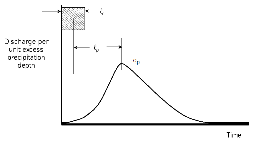
Thus, if t_r is specified, t_p can be calculated. If the duration of the desired unit hydrograph for the watershed of interest is significantly different than Equation 1, the following relationship can be used:

2)	$\begin{array}{l}\displaystyle t_{p R}=t_{p}-\frac{t_{r}-t_{R}}{4}\end{array}$

where t_R = lag of the desired unit hydrograph [hours]. For the standard case, Snyder found that q_p can be computed as:

3)	$\begin{array}{l}\displaystyle q_p=\frac{640 * C_p}{t_p}\end{array}$

where C_p = a coefficient derived from gaged data in the same region. For the non-standard case, the peak discharge per unit area of a desired unit hydrograph, q_pR, can be computed as:

4)	$\begin{array}{l}\displaystyle q_{pR}=\frac{640 * C_p}{t_R}\end{array}$

In the case of a standard unit hydrograph, Equation 1 and Equation 3 can then be solved to determine t_p and q_p. In the non-standard case, Equation 2 and Equation 4 can be used to determine t_p and q_p. As a final step, a curve with a unit depth of runoff must be fit through the previously computed ordinates. Snyder proposed a relationship with which the total time base of the unit hydrograph could be defined.

Instead of this relationship, within HEC-HMS, an equivalent Clark synthetic unit hydrograph is determined through an optimization routine and utilized in subsequent precipitation-runoff computations.

Required Parameters

Parameters that are required to utilize the “Standard” Snyder method within HEC-HMS include t_p [hours] and C_p. The most typical approach used to estimate the aforementioned parameters is through multi-linear regression analyses using various watershed physical characteristics and combinations. To utilize the “Ft Worth District” method, the total length along the stream centerline to the most hydraulically remote point [mi or km], the length along the stream centerline to the subbasin centroid [mi or km], the weighted slope between points along the stream centerline at 10- and 85-percent of the total length [ft/mi or m/km], percent urbanization, and percent sand must also be specified. To utilize the “Tulsa District” method, the total length along the stream centerline to the most hydraulically remote point [mi or km], the length along the stream centerline to the subbasin centroid [mi or km], the weighted slope between points along the stream centerline at 10- and 85-percent of the total length [ft/mi or m/km], and the percent channelization must also be specified. Typically, these values are estimated using GIS.

Estimating Parameters

Snyder collected rainfall and runoff data from gaged watersheds, derived the unit hydrograph as described earlier, parameterized these unit hydrograph, and related the parameters to measurable watershed characteristics. For the unit hydrograph lag, he proposed:

5)	$\begin{array}{l}\displaystyle t_{p}=C C_{t}\left(L L_{c}\right)^{0.3}\end{array}$

where Ct = basin coefficient; L = length of the main stream from the outlet to the divide; Lc = length along the main stream from the outlet to a point nearest the watershed centroid; and C = a conversion constant (0.75 for SI and 1.00 for foot-pound system). The parameter Ct of Equation 34 and Cp of Equation 32 are best found via calibration, as they are not physically-based parameters. Bedient and Huber (1992) report that Ct typically ranges from 1.8 to 2.2, although it has been found to vary from 0.4 in mountainous areas to 8.0 along the Gulf of Mexico. They report also that Cp ranges from 0.4 to 0.8, where larger values of Cp are associated with smaller values of Ct.
Alternative forms of the parameter predictive equations have been proposed. For example, the Los Angeles District, USACE (1944) has proposed to estimate tp as:

6)	$\begin{array}{l}\displaystyle t_{p}=C C_{t}\left(\frac{L L_{c}}{\sqrt{S}}\right)^{N}\end{array}$

where S = overall slope of longest watercourse from point of concentration to the boundary of drainage basin; and N = an exponent, commonly taken as 0.33. Others have proposed estimating tp as a function of tc , the watershed time of concentration (Cudworth, 1989; USACE, 1987). Time of concentration is the time of flow from the most hydraulically remote point in the watershed to the watershed outlet, and may be estimated with simple models of the hydraulic processes. Various studies estimate tp as 50-75% of tc.