Download PDF
Download page Selecting a Loss Method.
Selecting a Loss Method
While a subbasin element conceptually represents infiltration, surface runoff, and subsurface processes interacting together, the actual infiltration calculations are performed by a loss method contained within the subbasin. A total of twelve different loss methods are provided. Some of the methods are designed primarily for simulating events while others are intended for continuous simulation. All of the methods conserve mass. That is, the sum of infiltration and precipitation left on the surface will always be equal to total incoming precipitation. The suitability of the various methods for event and continuous simulation is shown in Table 1.
Table 1. Selecting a loss method for event or continuous simulation.
Loss Method | Event | Continuous |
|---|---|---|
| Deficit and constant | Yes | |
| Exponential | Yes | |
| Green and Ampt | Yes | |
| Gridded deficit and constant | Yes | |
| Gridded Green and Ampt | Yes | |
| Gridded SCS curve number | Yes | |
| Gridded soil moisture accounting | Yes | |
| Initial and constant | Yes | |
| Layered Green and Ampt | Yes | |
| SCS curve number | Yes | |
| Smith Parlange | Yes | |
| Soil moisture accounting | Yes |
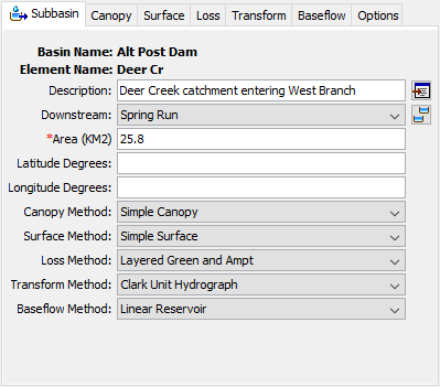
The loss method for a subbasin is selected on the Component Editor for the subbasin element as shown in Figure 1. Access the Component Editor by clicking the subbasin element icon on the "Components" tab of the Watershed Explorer. You can also access the Component Editor by clicking on the element icon in the basin map, if the map is currently open. You can select a loss method from the list of twelve available choices. If you choose the None method, the subbasin will not compute infiltration and all precipitation will be assumed as excess and subject to surface storage and runoff. Use the selection list to choose the method you wish to use. Each subbasin may use a different method or several subbasins may use the same method.
When a new subbasin is created, it is automatically set to use the default loss method specified in the program settings. You may change the loss method for a subbasin at any time using the Component Editor for the subbasin element. Since a subbasin can only use one loss method at a time, you will be warned when changing methods that the old parameter data will be lost. You can turn off this warning in the program settings. You can change the loss method for several subbasins simultaneously. Click on the Parameters menu and select the Loss | Change Method command. The loss method you choose will be applied to the selected subbasins in the basin model, or to all subbasins if none are currently selected.
The parameters for each loss method are presented on a separate Component Editor from the subbasin element editor. The "Loss" editor is always shown next to the "Surface" editor. If the kinematic wave transform method is selected, there may be two loss editors, one for each runoff plane. The information shown on the loss editor will depend on which method is currently selected.
A Note on Parameter Estimation
The values presented in sources such as Engineer Manual 1110-2-1417 Flood-Runoff Analysis, the HEC-HMS Technical Reference Manual, and the Introduction to Loss Rate Tutorials represent initial estimates. Regardless of the source, these initial estimates must be calibrated and validated.
Deficit and Constant Loss
The deficit constant loss method uses a single soil layer to account for continuous changes in moisture content. Using the deficit constant method allows for continuous simulation. It should be used in combination with a canopy method that will extract water from the soil in response to potential evapo-transpiration computed in the meteorologic model. The soil layer will dry out between precipitation events as the canopy extracts soil water. There will be no soil water extraction unless a canopy method is selected. It may also be used in combination with a surface method that will hold water on the land surface. The water in surface storage infiltrates to the soil layer. The infiltration rate is determined by the capacity of the soil layer to accept water. When both a canopy and surface method are used in combination with the deficit constant loss method, the system can be conceptualized as shown in Figure 2.
Precipitation fills the canopy storage. Precipitation that exceeds the canopy storage will overflow onto the land surface. The new precipitation is added to any water already in surface storage. If the moisture deficit is greater than zero, then water will infiltrate from the surface into the soil layer at a rate that is essentially infinite. This unlimited infiltration will continue until the soil layer reaches saturation (moisture deficit drops to zero) and during this period there is no percolation. The infiltration rate is defined by the constant rate while the soil layer remains at saturation. The percolation rate out the bottom of the layer is also defined by the constant rate while the soil layer remains at saturation. Percolation stops as soon as the soil layer drops below saturation (moisture deficit greater than zero). Moisture deficit increases in response to the canopy extracting soil water to meet the potential evapo-transpiration demand. The Component Editor is shown in Figure 3.
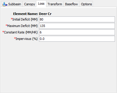
The initial deficit is the initial condition for the method. At the start of the simulation, it is the amount of water that would be required in order to fill the soil layer to the maximum storage.
The maximum deficit specifies the total amount of water the soil layer can hold, specified as an effective depth. An upper bound is the bulk thickness of the active soil layer multiplied by the porosity. However, in most cases such an estimate must be reduced by the permanent wilting point and for other conditions that reduce the water holding capacity. The thickness of the active soil layer is best determined through calibration.
The constant rate defines the infiltration and percolation rates when the soil layer is saturated. Saturated hydraulic conductivity is a good approximation.
The percentage of the subbasin which is directly connected impervious area can be specified. No loss calculations are carried out on the impervious area; all precipitation on that portion of the subbasin becomes excess precipitation and subject to surface storage and direct runoff.
Exponential Loss
The exponential loss method is empirical and generally speaking should not be used without calibration. The exponential loss method should only be used for event simulation. It represents incremental infiltration as an exponentially decreasing function of accumulated infiltration. It includes the option for increased initial infiltration when the soil is particularly dry before the arrival of a storm. Before using this method, consideration should be given to the Green and Ampt method because it produces a similar exponential decrease in infiltration and uses parameters with better physical interpretation. The Component Editor is shown in Figure 4.
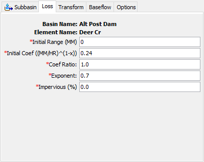
The initial range is the amount of initial accumulated infiltration during which the loss rate is increased. This parameter is considered to be a function primarily of antecedent soil moisture deficiency and is usually storm-dependent.
The initial coefficient specifies the starting loss rate coefficient on the exponential infiltration curve. It is assumed to be a function of infiltration characteristics and consequently may be correlated with soil type, land use, vegetation cover, and other properties of a subbasin.
The coefficient ratio indicates the rate at which the exponential decrease in infiltration capability proceeds. It may be considered a function of the ability of the surface of a subbasin to absorb precipitation and should be reasonably constant for large, homogeneous areas.
The precipitation exponent reflects the influence of precipitation rate on subbasin-average loss characteristics. It reflects the manner in which storms occur within an area and may be considered a characteristic of a particular region. It varies from 0.0 up to 1.0.
The percentage of the subbasin which is directly connected impervious area can be specified. No loss calculations are carried out on the impervious area; all precipitation on that portion of the subbasin becomes excess precipitation and subject to direct runoff.
Green and Ampt Loss
The Green Ampt infiltration method is essentially a simplification of the comprehensive Richard's equation for unsteady water flow in soil. The Green Ampt method should only be used for event simulation and not for a continuous simulation where there is an extended dry period(s) between precipitation. It assumes the soil is initially at uniform moisture content, and infiltration takes place with so-called piston displacement. It is also assumed that the soil layer is infinitely deep so that reaching saturation can be defined purely by the Green and Ampt equation. The method automatically accounts for ponding at the soil-air interface. The Component Editor is shown in Figure 5.
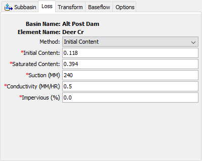
A method for specifying the initial soil moisture state at the beginning of a simulation must be selected. Two choices are available: Initial Content and Initial Deficit. The Initial Content method allows the user to specify the initial soil moisture state in terms of a moisture content. The two required parameters, initial content and saturated content, must be specified as volume ratios. Conversely, the Initial Deficit method allows the user to specify the initial soil moisture state in terms of a deficit. The single required parameter, initial deficit, must be specified as a volume ratio. The initial deficit can be calculated as the difference between the saturated content and initial content.
The saturated water content specifies the maximum water holding capacity in terms of volume ratio. It is often assumed to be the total porosity of the soil.
The wetting front suction must be specified. It is generally assumed to be a function of the soil texture.
The hydraulic conductivity must also be specified. It can be estimated from field tests or approximated by knowing the soil texture.
The percentage of the subbasin which is directly connected impervious area can be specified. No loss calculations are carried out on the impervious area; all precipitation on that portion of the subbasin becomes excess precipitation and subject to direct runoff.
Gridded Deficit Constant Loss
The gridded deficit constant loss method essentially implements the deficit constant method on a grid cell by grid cell basis. Each grid cell receives separate precipitation and potential evapotranspiration from the meteorologic model, while parameters are represented with grids from the grid data manager. A gridded canopy method should be selected that will extract water from the soil in response to potential evapo-transpiration computed in the meteorologic model. There will be no soil water extraction unless a canopy method is selected. The Component Editor is shown in Figure 6.
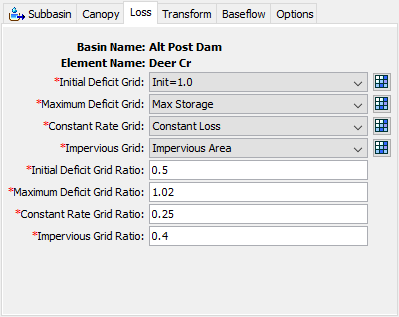
An initial deficit grid must be selected from the list of choices. The selection list will show all moisture deficit grids available in the grid data manager. You can use a chooser to select a grid by pressing the grid button next to the selection list. The chooser shows all of the moisture deficit grids in the grid data manager. Click on a grid to view the description. This is especially helpful since initial deficit and maximum storage grids are both stored as moisture deficit grids.
A maximum deficit grid must be selected from the list of choices. The selection list will show all moisture deficit grids available in the grid data manager. You can use a chooser to select a grid by pressing the grid button next to the selection list. The chooser shows all of the moisture deficit grids in the grid data manager. Click on a grid to view the description. This is especially helpful since initial deficit and maximum storage grids are both stored as moisture deficit grids.
A constant rate grid must be selected from the list of choices. The selection list will show all percolation rate grids available in the grid data manager. You can use the chooser to select a grid by pressing the grid button next to the selection list, or select directly from the list of choices.
An impervious grid must be selected from the list of choices. The selection list will show all impervious area grids available in the grid data manager. You can use the chooser to select a grid by pressing the grid button next to the selection list.
The initial deficit grid ratio must be entered. The actual initial deficit value at each grid cell is obtained by multiplying the value obtained from the initial deficit grid by the specified ratio. The default value is 1.0.
The maximum deficit grid ratio must be entered. The actual maximum deficit value at each grid cell is obtained by multiplying the value obtained from the maximum deficit grid by the specified ratio. The default value is 1.0.
The constant rate grid ratio must be entered. The actual constant loss rate value at each grid cell is obtained by multiplying the value obtained from the constant rate grid by the specified ratio. The default value is 1.0.
The impervious grid ratio must be entered. The actual percentage of impervious area at each grid cell is obtained by multiplying the value obtained from the impervious grid by the specified ratio. The default value is 1.0.
Gridded Green and Ampt Loss
The gridded Green Ampt loss method essentially implements the Green Ampt method on a grid cell by grid cell basis. The gridded Green Ampt method should only be used for event simulation. Each grid cell receives separate precipitation from the meteorologic model. Parameters are represented with grids from the grid data manager. The Component Editor is shown in Figure 7.
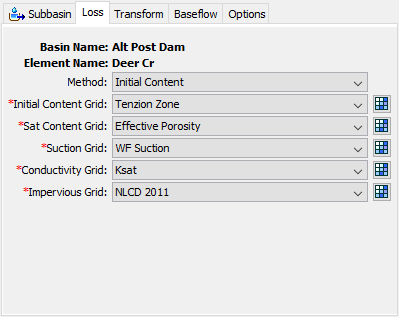
A method for specifying the initial soil moisture state at the beginning of a simulation must be selected. Two choices are available: Initial Content and Initial Deficit. The Initial Content method allows the user to specify the initial soil moisture state in terms of a moisture content. The two required parameters, initial content and saturated content, must be specified as volume ratios. Conversely, the Initial Deficit method allows the user to specify the initial soil moisture state in terms of a deficit. The single required parameter, initial deficit, must be specified as a volume ratio. The initial deficit can be calculated as the difference between the saturated content and initial content.
Depending upon the selected initial soil moisture state method, either an initial content and saturated content grid or just an initial deficit grid must be selected from the list of choices. All of the aforementioned grids are classified as water content grids. The selection list will show all water content grids available in the grid data manager. You can use the chooser to select a grid by pressing the grid button next to the selection list. The chooser shows all of the water content grids in the grid data manager. Click on a grid to view the description.
The wetting front suction grid must be selected from the list of choices. The selection list will show all of the water potential grids available in the grid data manager. You can use the chooser to select a grid by pressing the grid button next to the selection list.
The hydraulic conductivity grid must be selected from the list of choices. The selection list will show all of the percolation rate grids specified in the grid data manager, because conductivity is a type of percolation and has the same units. You can use the chooser to select a grid by pressing the grid button next to the selection list.
An impervious grid must be selected from the list of choices. The selection list will show all impervious area grids available in the grid data manager. You can use the chooser to select a grid by pressing the grid button next to the selection list.
Gridded SCS Curve Number Loss
The gridded SCS curve number loss method essentially implements the Soil Conservation Service (SCS) curve number method on a grid cell by grid cell basis. The gridded SCS curve number loss method should only be used for event simulation. Details of the curve number approach can be found in the National Engineering Handbook (NRCS, 2007). Each grid cell receives separate precipitation from the meteorologic model. All cells are initialized by scaling based on the curve number at each cell, and then allowed to evolve separately during the simulation based on individual precipitation inputs. The main parameter is represented with a grid from the grid data manager. The Component Editor is shown in Figure 8.
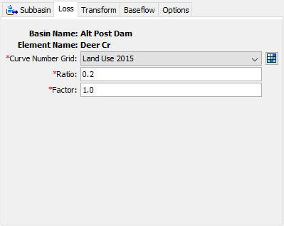
The curve number grid must be selected from the available choices. A curve number grid must be defined in the grid data manager before it can be used in the subbasin. You can use a chooser to select a grid by pressing the grid button next to the selection list. The chooser shows all of the curve number grids in the grid data manager.
The default initial abstraction ratio is 0.2 but may optionally be changed. The initial abstraction ratio is used to compute the initial abstraction at each grid cell. The potential retention is calculated from the curve number for each cell, then multiplied by the ratio to determine the actual initial abstraction for that cell.
The default potential retention scale factor is 1.0 but may optionally be changed. The potential retention scale factor is used to adjust the retention calculated from the curve number before it is multiplied by the initial abstraction ratio.
Gridded Soil Moisture Accounting Loss
The gridded soil moisture accounting loss method essentially implements the soil moisture accounting method on a grid cell by grid cell basis. Each grid cell receives separate precipitation and potential evapotranspiration from the meteorologic model. All cells are initialized to the same initial conditions, and then allowed to evolve separately during the simulation based on individual precipitation inputs. Parameters are specified on a cell by cell basis using grids from the grid data manager. A gridded canopy method should be selected that will extract water from the soil in response to potential evapo-transpiration computed in the meteorologic model. There will be no soil water extraction unless a canopy method is selected. The Component Editor is shown in Figure 9.
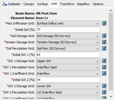
The maximum infiltration grid is selected from the percolation grids that have been previously defined in the grid data manager. The grid should specify the maximum infiltration rate at each grid cell. This is the upper bound on infiltration; the actual infiltration at any cell in a particular time interval is a linear function of the surface and soil storage in the cell, if a surface method is selected. Without a selected surface method, water will always infiltrate at the maximum rate. You may use a chooser to select the grid. The grid selections will be disabled unless you have previously created grids in the grid data manager. Likewise, you must also select a soil percolation and groundwater percolation grids. All infiltration and percolation grids use the same type of parameter grid so descriptions for the grids are important.
The initial condition of the soil should be specified as the percentage of the soil storage that is full of water at the beginning of the simulation. The same percentage will be applied to every grid cell. Likewise, you must specify the initial storage of each groundwater layer.
The soil storage grid must be selected from the grids that have been previously defined in the grid data manager. The grid should specify the maximum soil storage in each grid cell. You may use a chooser to select the grid by pressing the grid button next to the selection list. You will not be able to select a grid if no grids have been created in the grid data manager. Likewise, you must select a tension storage grid, and a storage grid for each groundwater layer. Because tension storage is contained within the total soil storage, the tension storage at each cell must be less than the soil storage at the same cell.
Groundwater coefficient grids must be selected for the upper and lower groundwater layers. The selected grid should specify the storage coefficient for each cell in the layer. The coefficient is used as the time lag on a linear reservoir for transforming water in storage to become lateral outflow. Contributions from each grid cell are accumulated to determine the total amount of flow available to become baseflow.
Initial and Constant Loss
The initial constant loss method is very simple but still appropriate for watersheds that lack detailed soil information. It is also suitable for certain types or flow-frequency studies. The initial constant loss method should only be used for event simulation. The Component Editor is shown in Figure 10.
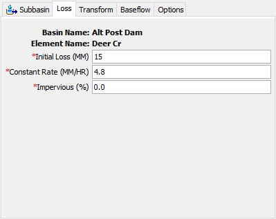
The initial loss specifies the amount of incoming precipitation that will be infiltrated or stored in the watershed before surface runoff begins. There is no recovery of the initial loss during periods without precipitation.
The constant rate determines the rate of infiltration that will occur after the initial loss is satisfied. The same rate is applied regardless of the length of the simulation.
The percentage of the subbasin which is directly connected impervious area can be specified. No loss calculations are carried out on the impervious area; all precipitation on that portion of the subbasin becomes excess precipitation and subject to direct runoff.
Layered Green and Ampt Loss
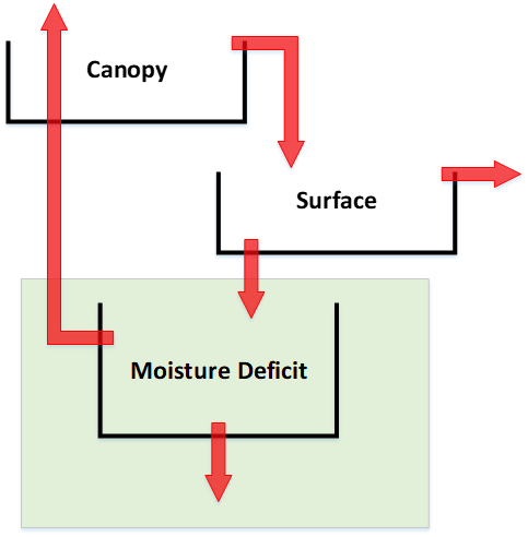
The layered Green Ampt loss method uses two soil layers to account for continuous changes in moisture content. The method is based on algorithms originally developed for the Guelph Agricultural Watershed Storm-Event Runoff (GAWSER) model. Using the layered Green Ampt method allows for continuous simulation. It should be used in combination with a canopy method that will extract water from the soil in response to potential evapo-transpiration computed in the meteorologic model. The soil layer will dry out between precipitation events as the canopy extracts soil water. There will be no soil water extraction unless a canopy method is selected. It may also be used in combination with a surface method that will hold water on the land surface. The water in surface storage infiltrates to the soil layer. The infiltration rate is determined by the capacity of the soil layer to accept water. When both a canopy and surface method are used in combination with the deficit constant loss method, the system can be conceptualized as shown in Figure 11.
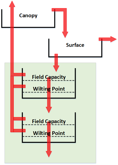
The layered Green Ampt loss method uses two layers to represent the dynamics of water movement in the soil. Surface water infiltrates into the upper layer, called layer 1. Layer 1 produces seepage to the lower layer, called layer 2. Both layers are functionally identical but may have separate and distinct parameters. Separate parameters can be used to represent layered soil profiles and also allows for better representation of stratified soil drying between storms. Each layer is described using a bulk depth and water content values for saturation, field capacity, and wilting point. Soil water in layer 2 can percolate out of the soil profile. The layered Green Ampt method is intended to be used in combination with the linear reservoir baseflow method. When used in this manner, the percolated water can be split between baseflow and aquifer recharge.
Precipitation fills the canopy storage. Precipitation that exceeds the canopy storage will overflow onto the land surface. The new precipitation is added to any water already in surface storage. The infiltration rate from the surface into layer 1 is calculated with the Green and Ampt equation so long as layer 1 is below saturation. The infiltration rate changes to the current seepage rate when layer 1 reaches saturation. Infiltration water is added to the storage in layer 1. Seepage out of layer 1 only occurs when the storage exceeds field capacity. Maximum seepage occurs when layer 1 is at saturation and declines to zero at field capacity. The seepage rate changes to the percolation rate when layer 2 is saturated. Seepage is added to the storage in layer 2. Percolation out of layer 2 only occurs when the storage exceeds field capacity. Maximum percolation occurs when layer 2 is at saturation and declines to zero at field capacity. Most soils observe decreasing hydraulic conductivity rates at greater depths below the surface. This means that typically the seepage rate is reduced to the percolation rate when layer 2 saturates, and the infiltration rate is reduced to the seepage rate when layer 1 saturates. The infiltration rate will change to the percolation rate if both layers 1 and 2 are saturated. Both convergence control and adaptive time stepping are used to accurately resolve the saturation of each layer.
The canopy extracts water from soil storage to meet the potential evapo-transpiration demand. First, soil water is extracted from layer 1 at the full evapo-transpiration rate. This extraction from layer 1 continues until half of the available water has been taken to meet the evapo-transpiration demand. The available water is defined as the saturation content minus the wilting point content, multiplied by the bulk layer thickness. Second, soil water is extracted from layer 2 at the full evapo-transpiration rate. This extraction from layer 2 also continues until half of the available water has been taken. Third, the evapo-transpiration demand is applied equally to both layers until one of them reaches wilting point content. Finally, the evapo-transpiration demand is applied to the remaining layer until it also reaches wilting point content. Soil water below the wilting point content is never used for evapo-transpiration.
The layered Green Ampt loss method can be used for continuous simulation because it is built on a water balance of the two layers. Infiltrated water is added to the layers and percolated water is removed from the layers. Potential evapo-transpiration demand also removes water from the layers. The continuous simulation will include storm events from time to time. The Green and Ampt equation is used to compute the surface infiltration during each of these storm events. The initial condition of the Green and Ampt equation for each of these storms must be determined. The initial content is essentially a water content deficit which can be calculated as the saturated water content minus the current water content. The water content deficit is automatically calculated at the beginning of each storm based on current soil water storage in layer 1. The user can control the amount of time that must pass since the last precipitation in order for the initial condition to be recalculated, using the dry duration parameter. When the time since last precipitation is less than the dry duration, the precipitation is considered a continuation of the last storm event. The Component Editor is shown in Figure 12.
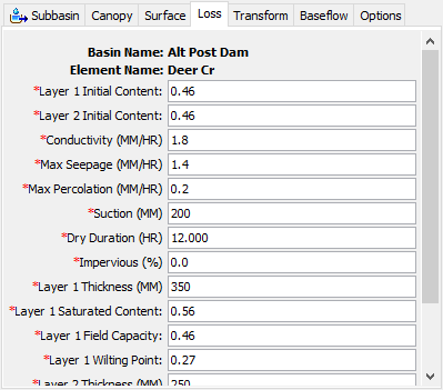
The layer 1 initial water content sets the amount of soil water at the beginning of a simulation. It should be specified in terms of volume ratio.
The layer 2 initial water content sets the amount of soil water at the beginning of a simulation. It should be specified in terms of volume ratio.
The hydraulic conductivity should be specified. It can be estimated from field tests or approximated by knowing the surface soil texture.
The maximum seepage must be specified at the bottom of layer 1. Field tests or the soil texture at the bottom of layer 1 can be used to estimate a value.
The maximum percolation must be specified at the bottom of layer 2. Field tests or the soil texture at the bottom of layer 2 can be used to estimate a value.
The wetting front suction must be specified. It is generally assumed to be a function of the soil texture.
The dry duration sets the amount of time that must pass after a storm event in order to recalculate the initial condition for the Green and Ampt equation. It has been found that 12 hours often works well.
The percentage of the subbasin which is directly connected impervious area can be specified. No loss calculations are carried out on the impervious area; all precipitation on that portion of the subbasin becomes excess precipitation and subject to direct runoff.
The layer 1 thickness sets the bulk depth of soil measured from the ground surface down to the bottom of layer 1.
The layer 1 saturated water content specifies the maximum water holding capacity in terms of volume ratio. It is often assumed to be the total porosity of the soil.
The layer 1 field capacity content specifies the point where the soil naturally stops seeping under gravity, in terms of volume ratio.
The layer 1 wilting point content specifies the amount of water remaining in the soil when plants are no longer capable of extracting it. It should be specified in terms of volume ratio.
The layer 2 thickness sets the bulk depth of soil measured from the bottom of layer 1 down to the bottom of layer 2.
The layer 2 saturated water content specifies the maximum water holding capacity in terms of volume ratio. It is often assumed to be the total porosity of the soil.
The layer 2 field capacity content specifies the point where the soil naturally stops percolating under gravity, in terms of volume ratio.
The layer 2 wilting point content specifies the amount of water remaining in the soil when plants are no longer capable of extracting it. It should be specified in terms of volume ratio.
SCS Curve Number Loss
The Soil Conservation Service (SCS) curve number method implements the curve number methodology for incremental losses (NRCS, 2007). The SCS curve number loss method should only be used for event simulation. Originally, the methodology was intended to calculate total infiltration during a storm. The program computes incremental precipitation during a storm by recalculating the infiltration volume at the end of each time interval. Infiltration during each time interval is the difference in volume at the end of two adjacent time intervals. The Component Editor is shown in Figure 13.
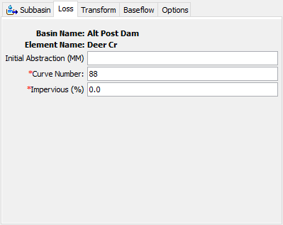
You may optionally enter an initial abstraction. The initial abstraction defines the amount of precipitation that must fall before surface excess results. However, it is not the same as an initial interception or initial loss since changing the initial abstraction changes the infiltration response later in the storm. If this value is left blank, it will be automatically calculated as 0.2 times the potential retention, which is calculated from the curve number.
You must enter a curve number. This should be a composite curve number that represents all of the different soil group and land use combinations in the subbasin. The composite curve number should not include any impervious area that will be specified separately as the percentage of impervious area.
The percentage of the subbasin which is directly connected impervious area can be specified. Any percentage specified should not be included in computing the composite curve number. No loss calculations are carried out on the impervious area; all precipitation on that portion of the subbasin becomes excess precipitation and subject to direct runoff.
Smith and Parlange Loss
The Smith Parlange loss method approximates Richard's equation for infiltration into soil by assuming the wetting front can be represented with an exponential scaling of the saturated conductivity. This linearization approach allows the infiltration computations to proceed very quickly while maintaining a reasonable approximation of the wetting front. The Smith Parlange loss method should only be used for event simulation. The Component Editor is shown in Figure 14.
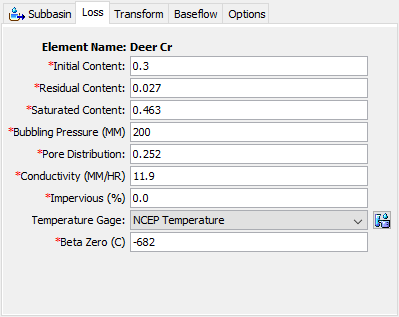
The initial water content gives the initial saturation of the soil at the beginning of a simulation. It should be specified in terms of volume ratio.
The residual water content specifies the amount of water remaining in the soil after all drainage has ceased. It should be specified in terms of volume ratio. It may be determined in the laboratory or estimated from the soil texture.
The saturated water content specifies the maximum water holding capacity in terms of volume ratio. It is often assumed to be the total porosity of the soil.
The bubbling pressure, also known as the wetting front suction, must be specified. It is generally assumed to be a function of the soil texture.
The pore size distribution determines how the total pore space is distributed in different size classes. It is typically assumed to be a function of soil texture.
The hydraulic conductivity must also be specified, typically as the effective saturated conductivity. It can be estimated from field tests or approximated by knowing the soil texture.
The percentage of the subbasin which is directly connected impervious area can be specified. No loss calculations are carried out on the impervious area; all precipitation on that portion of the subbasin becomes excess precipitation and subject to direct runoff.
Optionally, a temperature gage may be selected for adjusting the water density, water viscosity, and matric potential based on temperature. If no temperature gage is selected then a temperature of 25C (75F) is assumed to prevail. The gage must be defined in the time-series manager before it can be selected in the component editor.
The beta zero parameter is used to correct the matric potential based on temperature. It has been found to be a function of soil texture. It will only be shown for input if a temperature gage has been selected. Table 2 provides mean estimates of beta zero.
Table 2. Beta zero parameter values for various soil textures classes.
USDA Soil Texture | beta zero |
|---|---|
| Sand | -404.9 |
| Loamy sand | -403.4 |
| Sandy loam | -400.7 |
| Loam | -397.1 |
| Silt loam | -399.2 |
| Sandy clay loam | -393.5 |
| Clay loam | -390.4 |
| Silty clay loam | -390.0 |
| Sandy clay | -386.9 |
| Silty clay | -383.9 |
| Clay | -376.8 |
Soil Moisture Accounting Loss
The soil moisture accounting loss method uses three layers to account for continuous changes in moisture content throughout the vertical profile of the soil. Using the soil moisture accounting method allows for continuous simulation. It should be used in combination with a canopy method that will extract water from the soil in response to potential evapo-transpiration computed in the meteorologic model. The soil layer will dry out between precipitation events as the canopy extracts soil water. There will be no soil water extraction unless a canopy method is selected. It may also be used in combination with a surface method that will hold water on the land surface. The water in surface storage infiltrates to the soil layer. The infiltration rate is determined by the capacity of the soil layer to accept water. When both a canopy and surface method are used in combination with the soil moisture accounting loss method, the system can be conceptualized as shown in Figure 15.
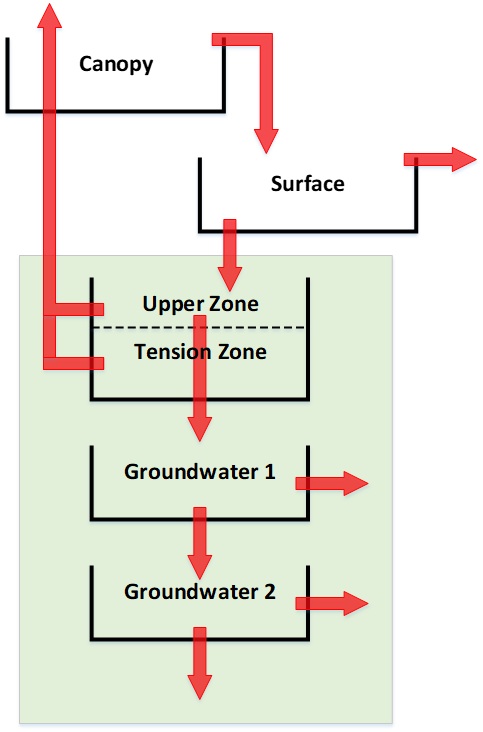
The soil moisture accounting loss method uses three layers to represent the dynamics of water movement in the soil. Layers include soil storage, upper groundwater, and lower groundwater. Groundwater layers are not designed to represent aquifer processes; they are intended to be used for representing shallow inter-flow processes. The soil layer is subdivided into an upper zone and a tension zone. Soil water only percolates from the upper zone while water in the tension zone resists percolation. Water in upper groundwater percolates to lower groundwater. The soil moisture accounting loss method is designed to be used in combination with the linear reservoir baseflow method. When used in this way, water can move laterally out of upper groundwater and lower groundwater to enter baseflow. Water percolating out of lower groundwater can be split between entering baseflow and leaving the land surface as aquifer recharge.
Precipitation fills the canopy storage. Precipitation that exceeds the canopy storage will overflow onto the land surface. The new precipitation is added to any water already in surface storage. The current infiltration rate is a function of the maximum infiltration rate, the current surface storage, and the current soil storage. The highest infiltration occurs when the surface storage is at maximum and the soil storage is at zero. Infiltration approaches zero as the surface storage falls to zero or as the soil storage reaches saturation. Infiltration water is added to the water already in soil storage. The upper zone and tension zone both exist within the soil storage. Water will percolate from the soil to upper groundwater whenever the soil storage is between the tension zone depth and the soil storage depth. The percolation rate is a function of the maximum percolation rate, the current soil storage, and the current upper groundwater storage. The highest percolation occurs when the soil storage is at maximum (saturated) and the upper groundwater is at zero. Percolation approaches zero as the soil storage falls to the tension zone depth or as the groundwater reaches saturation. Similarly, water percolates from upper groundwater to lower groundwater as a function of the maximum upper groundwater percolation rate, the upper groundwater storage, and the lower groundwater storage.
The canopy extracts water from soil storage to meet the potential evapo-transpiration demand. Soil water is extracted from the upper zone at the full potential evapo-transpiration rate. Once soil storage falls to the tension storage depth, the further extraction of soil water is determined by the interaction of the canopy and the amount of water in soil storage. This interaction is configured in the canopy component as the plant uptake method. Depending on the uptake method, water may be extracted from the soil at the full potential evapo-transpiration rate until no water remains in soil storage. An alternate uptake method continues to extract water at the full potential evapo-transpiration rate until soil water falls to half of the tension storage depth, with extraction less than potential as soil storage falls to zero. Potential evapo-transpiration is never extracted from the groundwater layers. The Component Editor is shown in Figure 16.
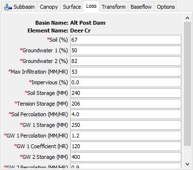
The initial condition of the soil should be specified as the percentage of the soil that is full of water at the beginning of the simulation. The initial condition of the upper and lower groundwater layers must also be specified.
The maximum infiltration rate sets the upper bound on infiltration from the surface storage into the soil. This is the upper bound on infiltration; the actual infiltration in a particular time interval is a linear function of the surface and soil storage, if a surface method is selected. Without a selected surface method, water will always infiltrate at the maximum rate.
The percentage of the subbasin which is directly connected impervious area can be specified. All precipitation on that portion of the subbasin becomes excess precipitation and subject to direct runoff.
Soil storage represents the total storage available in the soil layer. It may be zero if you wish to eliminate soil calculations and pass infiltrated water directly to groundwater.
Tension storage specifies the amount of water storage in the soil that does not drain under the affects of gravity. Percolation from the soil layer to the upper groundwater layer will occur whenever the current soil storage exceeds the tension storage. Water in tension storage is only removed by evapotranspiration. By definition, tension storage must be less that soil storage.
The soil percolation sets the upper bound on percolation from the soil storage into the upper groundwater. The actual percolation rate is a linear function of the current storage in the soil and the current storage in the upper groundwater.
Groundwater 1 storage represents the total storage in the upper groundwater layer. It may be zero if you wish to eliminate the upper groundwater layer and pass water percolated from the soil directly to the lower groundwater layer.
The groundwater 1 percolation rate sets the upper bound on percolation from the upper groundwater into the lower groundwater. The actual percolation rate is a linear function of the current storage in the upper and lower groundwater layers.
The groundwater 1 coefficient is used as the time lag on a linear reservoir for transforming water in storage to become lateral outflow. The lateral outflow is available to become baseflow.
Groundwater 2 storage represents the total storage in the lower groundwater layer. It may be zero if you wish to eliminate the lower groundwater layer and pass water percolated from the upper groundwater layer directly to deep percolation.
The groundwater 2 percolation rate sets the upper bound on deep percolation out of the system. The actual percolation rate is a linear function of the current storage in the lower groundwater layer.
The groundwater 2 coefficient is used as the time lag on a linear reservoir for transforming water in storage to become lateral outflow. It is usually a larger value that the groundwater 1 coefficient. The lateral outflow is likewise available to become baseflow.