Elements in the basin model can be designated as computation points. Generally only elements with observed flow, observed stage, or other observed data are designated as computation points. Computation points are designed primarily for use with simulation runs and forecast alternatives. When used with a simulation run, the features of a computation point are a customizable editor that uses slider bars to adjust parameters upstream of the computation point, and result graphs with customizable time-series selection. Results from the simulation run are automatically recomputed as the slider bars are adjusted and the result graphs update dynamically. When used with forecast alternatives, the principal feature of a computation point is to make upstream to downstream calibration more efficient.

Selecting Computation Points

Any element in the basin model can be selected as a computation point, and there is no limit to the number of computation points permitted. Usually an element is only designated as a computation point if it includes observed data that can aid in calibration. However, observed data is not absolutely necessary.

There are two ways to select an element as a computation point. The first way is to click on the element in the Basin Model Map window using the right mouse button (Figure 1). Choose the Select Computation Point command to select the element as a computation point. It is only possible to select the element as a computation point if it is not already selected. An element selected as a computation point shows a small red circle added to the icon in the Basin Model Map window and also in the Watershed Explorer.

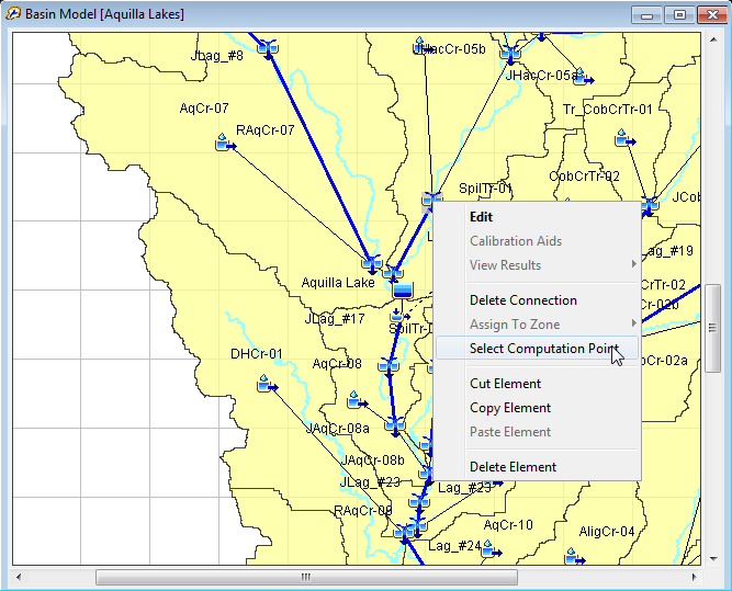
Figure 1. Setting a junction to be a computation point by right-clicking in the basin model map.

The second way to select an element as a computation point is by using the Computation Point Manager window (Figure 2). To access the manager, click on the Parameters menu and choose the Computation Point Manager command. The manager shows all of the elements that have been selected as computation points. Press the Select Elements button to begin the process of selecting an element as a computation point. The Select Elements window (Figure 3) includes a selection list for choosing the type of element to display in the selection table. The selection table shows the element name and description for all elements in the basin model that match the selected element type. By default only elements with observed data are shown in the table, but all elements can be shown by using the option in the upper right of the window. To select an element as a computation point, click on the row in the table and press the Select button. You cannot make a selection unless a row in the table is selected; the selected row in the table is highlighted. Press the Close button when you are done selecting elements and you will return to the Computation Point Manager window.

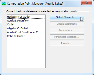
Figure 2. The computation point manager.

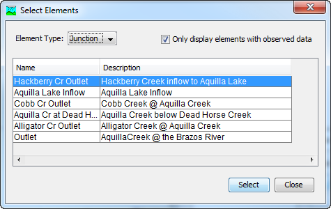
Figure 3. Selecting elements to be computation points. The element type is set to show only junctions, and the observed data option limits the elements to those with observed flow, observed stage, or another type of observed data.

Unselecting Computation Points

There are two ways to unselect an element so that it is no longer a computation point. The first way is to click on the element in the Basin Model Map window using the right mouse button (Figure 4). Choose the Unselect Computation Point command to indicate the element will no longer be a computation point. It is only possible to unselect the element if it is already selected as a computation point. The small red circle added to the element icon in the Basin Model Map window and also in the Watershed Explorer will be removed to indicate the element is no longer a computation point.

The second way to unselect an element as a computation point is by using the Computation Point Manager window (Figure 5). To access the manager, click on the Parameters menu and choose the Computation Point Manager command. The manager shows all of the elements that have been selected as computation points. Select the element that will discontinue as a computation point; the selected element is highlighted in the list. Press the Unselect Element button to undesignate the selected element as a computation point.

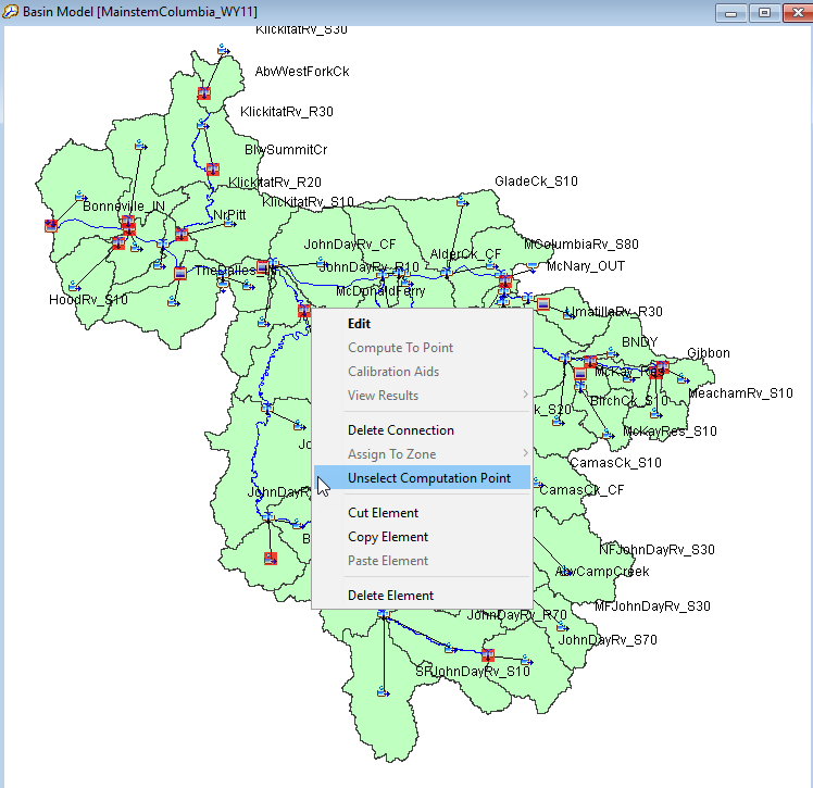
Figure 4. Setting a junction to no longer be a computation point by right-clicking in the basin model map.

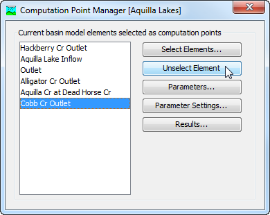
Figure 5. Unselecting an element as a computation point using the computation point manager.

Selecting Calibration Parameters

Each computation point includes a customizable editor to aid in calibration of a simulation run. The editor can be customized by selecting the parameters it will contain. The parameters selected for the editor must be in the elements upstream of the computation point. If the computation point is a subbasin or reach element, then parameters at that element may also be selected. If there is an upstream computation point, then the selected parameters must be at elements between the two computation points. Parameters selected at one computation point will be automatically transferred if a new computation point is selected upstream.

The process of selecting parameters for the customizable editor at a computation point begins on the Computation Point Manager window (Figure 6). To access the manager, click on the Parameters menu and choose the Computation Point Manager command. The manager shows all of the elements that have been selected as computation points. Select the computation point where you wish to add parameters; the selected computation point is highlighted in the list. Press the Parameters… button open the parameter management window (Figure 7) and then press the Select… button to begin selecting the parameters for the computation point.

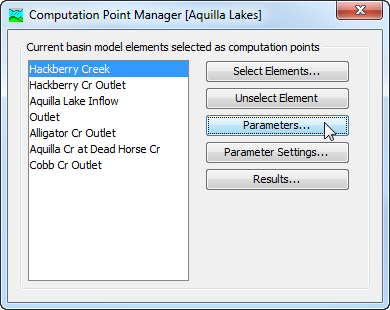
Figure 6. Preparing to select parameters for the customizable editor at the "Hackberry Creek" computation point.

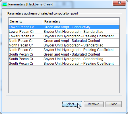
Figure 7. The parameters management window shows all the parameters for a computation point selected in the Computation Point Manager.

The Select Parameters window is used to choose the parameters to add to a computation point. Each of the subbasin and reach elements upstream of the computation point are shown in a list on the left side of the window. The element selected as the computation point is also shown in the list if the element is a subbasin or reach. Click on an element in the list on the left side of the window; the selected element is highlighted. The right side of the window will be updated to show all of the parameters at the selected element that can be chosen for the customizable editor (Figure 8). More than one parameter can be selected simultaneously by holding the control key and clicking on several parameters. Press the Select button when you have selected the parameters you wish to add. Selected parameters are removed from the list of available parameters. You can choose parameters from additional elements by clicking on each element in the list on the left side of the window and selecting parameters from that element. When you are finished selecting parameters for the computation point, press the Close button to return to the Parameters window.

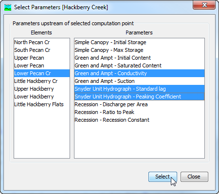
Figure 8. Selecting parameters for a computation point from those available at a subbasin element. Hold the control key and click with the mouse to select multiple parameters simultaneously.

Unselecting Calibration Parameters

Begin unselecting parameters from the customizable editor at a computation point using the the Computation Point Manager window (Figure 6). To access the manager, click on the Parameters menu and choose the Computation Point Manager command. The manager shows all of the elements that have been selected as computation points. Select the computation point where you wish to remove parameters; the selected computation point is highlighted in the list. Press the Parameters.. button to begin removing parameters from the computation point.

The Parameters window shows all parameters that have been selected at the computation point. The left column in the table shows the name of the element and the right column in the table shows the parameter. The parameter is specified with the name of the method followed by the name of the parameter. In the example shown in Figure 9, the first row in the table represents the "Conductivity" parameter in the "Green Ampt" loss rate method of subbasin "Lower Pecan Cr." Click a row in the table to select it; the selected row is highlighted. Press the Remove button to remove the parameter from the computation point. You may unselect more than one parameter at a time by holding the control key and clicking on multiple rows in the table. Press the Close button when you have finished unselecting parameters and you will return to the Computation Point Manager window.

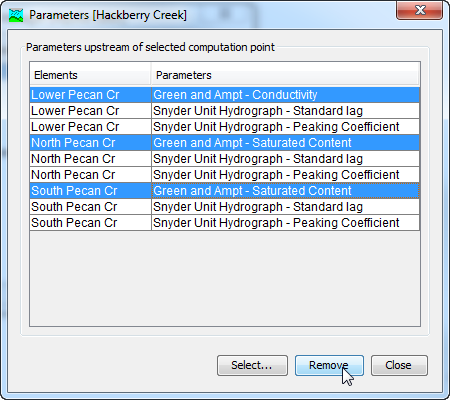
Figure 9. Unselecting parameters from a computation point. Hold the control key to select multiple parameters to be unselected.

Settings for Calibration Parameters

The parameters in the customizable editor are represented with slider bars. The slider can be used to quickly change each parameter value in the range from a minimum value to a maximum value. By default the minimum and maximum values cover a very wide range. You can change the minimum and maximum values for each parameter to narrow the adjustment range to be suitable for a particular subbasin or reach in a watershed.

Change parameter settings for the customizable editor at a computation point using the Computation Point Manager window (Figure 6). To access the manager, click on the Parameters menu and choose the Computation Point Manager command. The manager shows all of the elements that have been selected as computation points. Select the computation point where you wish to make the parameter settings; the selected computation point is highlighted in the list. Press the Parameter Settings button to begin editing the parameter settings for the computation point.

The Parameter Settings window shows all of the parameters selected at a computation point. Each row in the table displays settings information for one parameter. The first column specifies the name of the element. The second column specifies the name of the method followed by the name of the parameter. The third column specifies the units of the parameter. In the example shown in Figure 10, the first row in the table represents the "Standard Lag" parameter in the "Snyder" transform method of subbasin "Lower Pecan Cr." The units of the parameter are "HR" which represents hours. You may specify the minimum and maximum value for the parameter in the final two columns of the table. While the parameter may take on values less than the minimum or greater than the maximum, the slider bar in the customizable editor for the computation point will only be able to adjust the parameter value within the range specified in the table.

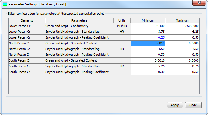
Figure 10. Changing the minimum and maximum parameter values in the customizable editor at a computation point.

Computation Point Results

A computation point may optionally include up to five customized result graphs. You may specify which time-series results appear in each graph. The results selected for a graph must be in the elements upstream of the computation point, or at the computation point itself. If there is an upstream computation point, then the selected parameters must be at elements between the two computation points. Any of the various time-series computed at an element may be included in a graph. The results in the graphs will automatically update as soon as adjustments are made to parameter values using the customizable editor at the computation point.

Configure results at a computation point using the the Computation Point Manager window (Figure 6). To access the manager, click on the Parameters menu and choose the Computation Point Manager command. The manager shows all of the elements that have been selected as computation points. Select the computation point where you wish to configure result graphs; the selected computation point is highlighted in the list. Press the Results button to begin configuring the results for the computation point. The Results window opens and allows you to configure the results for up to five graphs (Figure 11). The selector in the upper left allows you to choose which graph to configure; you may select any of the five graphs. The table in the center of the window shows all of the results for the selected graph. The element name and the result name are shown for each result added to the graph.

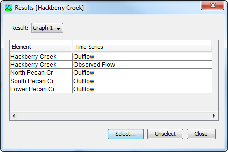
Figure 11. Selected results for the first graph at computation point "Hackberry Creek." The outflow and observed flow are included from the computation point, plus the outflow from several upstream subbasins.

Add a result to a graph by pressing the Select button in the Results window. The Select Time-Series window opens for choosing one or more results to add to the current graph selection (Figure 12). The left side of the window shows the computation point element and all elements upstream of it. Select the element that produces the result that you wish to add to the graph. Select the element by clicking on it with the mouse; the selected element is highlighted in the list. Only one element can be selected at a time. All of the available time-series for the selected element are shown on the right side. Select the time-series result you wish to add to the graph by clicking on it and then pressing the Select button. You can add multiple time-series results simultaneously by holding the control key and clicking on more than one result. All selected time-series are added to the graph when the Select button is pressed. Time-series results are not shown in the list if they have already been added to the graph. Press the Close button when you are done selecting results and wish to return to the Results window.

Remove a selected time-series result from a graph directly on the Results window (Figure 13). Select the result you wish to remove by clicking it with the mouse; the selected result is highlighted in the list. You may select multiple results simultaneously by holding the control key and clicking additional results. Press the Unselect button to remove the time-series results from the current graph selection.

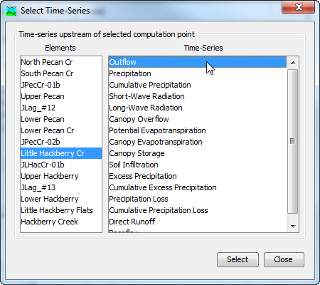
Figure 12. Selecting the outflow time-series from a subbasin element for addition to a result graph at a computation point. Multiple time-series can be selected simultaneously by holding the control key and selecting additional time-series results.

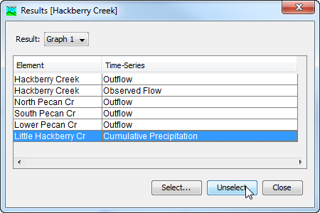
Figure 13. Removing a time-series result from a graph at a computation point.