There are several sediment transport options which are only available in 2D. The goal is for both 1D and 2D sediment transport to have the same options but for now the 2D only options have been places in a single editor called 2D Options which is available from the Sediment Data editor under the Options menu.  The 2D Sediment Options editor is shown in the figure below. The editor is used to specify the options for sheet and splash erosion, the morphologic acceleration factor, the base bed-slope coefficient, and hindered settling.

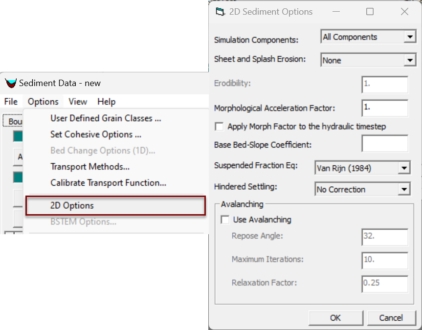
Figure. 2D Options editor from the Sediment Data editor.

Simulation Components

HEC-RAS 2D Sediment has 5 simulation modes which turn on and off different simulation components.  The default, All Components, engages the full, advection-diffusion, mobile-bed model with all components of the transport equation, bed-change equation, and updates to the cell gradation and bed elevations.  Each of the other modes is a simplification of that full suite, to provide intermediate-complexity analyses.  HEC recommends starting with these lower complexity approaches and adding complexity incrementally.  

Figure. 2D Simulation Components.

Capacity Only

Capacity Only computes only the sediment transport capacity (i.e. equilibrium concentrations) for all grain classes and does not solve the transport, bed sorting, and bed layering equations. Transport rates are computed with the sediment capacity equations. The Capacity Only option is essentially a hydraulic post processor and runs much faster because it does not solve transport, bed sorting, and bed layering equations for each grain class.  Run times should be similar to the hydraulic simulation.  This makes the method very useful for screening sediment transport functions and estimating initial sediment bed gradations and sediment boundary conditions.  The Guides and Tutorials include a Capacity only tutorial and video.

Capacity only is sensitive to the bed material (because it uses the bed material to apportion transport capacity to the grain classes) but is not sensitive to sediment boundary conditions because it does not transport sediment between cells.  The transport equations are included below with the components excluded from this analysis greyed out.  Only the equilibrium concentration (which comes from the transport capacity equations) is active.

Concentration Only

The Concentration Only option simulation solves the advection-diffusion transport equation but does not simulate any bed processes (see governing equations below). 

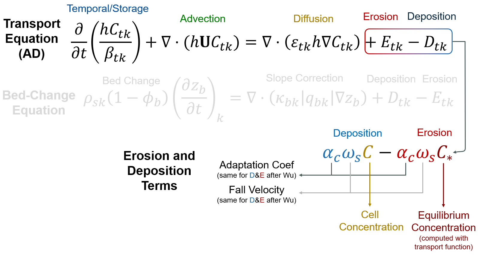
The Concentration Only option requires sediment boundary conditions because it will transport the boundary concentrations through the model.   The erosion and deposition terms are also active, so each cell can either gain or lose sediment from or to the bed based on fall velocity (deposition) or equilibrium concentration (erosion).  Users can exclude the erosion term by setting the calibration multiplier or the erosion scaling factor to further simplify this into a non-erodible model (e.g. concentration-only/deposition-only) which can be a useful simplification because erosion is a more empirical and uncertain process than deposition. 

Gradation (no Elev) and Bed Elev (no Grad)

 These methods run the full mobile bed model but only change one component of the bed (gradation or bed elevation).  The Gradation (no Elev) simulation components option simulates sediment concentrations and bed sorting and layering but keeps the bed elevations constant. The Bed Elev (no Grad) option simulations sediment concentrations and bed change but does not change the bed gradations. 

These are generally used model preconditioning and hot starts.  By holding one aspect of the bed fixed and allowing the other to evolve, the model can often achieve an appropriate starting condition.

Sheet and Splash Erosion

The first option available in the editor is the Sheet and Splash Erosion. The 2D sediment transport model has the option to use the Wei et al. (2009). The formulation has an erodibility coefficient which for simplicity is set to a single value in HEC-RAS. The units of the erodibility coefficient are kg∙m^-3.644∙s^0.644. Wei et al. (2009) reported values for the sheet and splash erosion coefficient between 1124 and 2555 kg∙m^-3.644∙s^0.644 for 3 grassland rangeland plots in Arizona (all variables in the International System of Units). However, its value can vary by orders of magnitude for different soil types and cover characteristics.

Morphologic Acceleration Factor

As the name implies, the Morphologic Acceleration Factor (Morp Fact) can accelerate model bed change. The factor is directly multiplied by the mass bed exchange rates at every time step. A value of zero will turn off the bed elevation and bed composition change but a factor of 2, for example, will double it.

The Morphologic Acceleration Factor is usually a scaling factor for bed change. This approach is commonly used in coastal applications with tidal boundary conditions. For example, running a 5-year simulation with Morphologic Acceleration Factor of 6 can approximate 30 years of change, which greatly reduces the computational time. However, while Morphological Acceleration does maintain sediment feedbacks between time steps, it changes the order of events (i.e. storms and tidal forcing with respect to morphological features) which can be important in bed change analysis and affects the accuracy of the results.

If this is a new model and/or the flow data are specified with the correct time interval, make sure the Apply Morph Factor to the hydraulic time step check box is selected.  This will automatically manage time compression for input and output (so you do not have to change your flow time series). 

This option is not selected by default.  Make sure you check this box for any new model.

Legacy Guidence for Time Series Compression (if the hydraulic timestep option is not checked)

Changing the Boundary Condition Time Step with the Morphological Acceleration Factor

Prior to version 6.7, users had to compress their time series proportional to the morphological acceleration for Morphologically Accelerated results to make sense temporally.  In version 6.7 HEC added logic to HEC-RAS to compress and decompress time automatically based on your morphological acceleration.  If you check the  Apply Morph Factor to the hydraulic time step option, you should not need to change your time series.

But we include the process below for how users used to compress their flow time series in case you are working with a legacy model that did this (and do not check the box).

It is useful to choose a Morphological Acceleration Factor that is easily divisible by the time step.  For example, if a boundary condition data increment is 15 minutes, selecting Morphological Acceleration Factors of 3, 5, or, 15 makes it easier to adjust these data to accommodate the temporal dilation.  See these three examples below: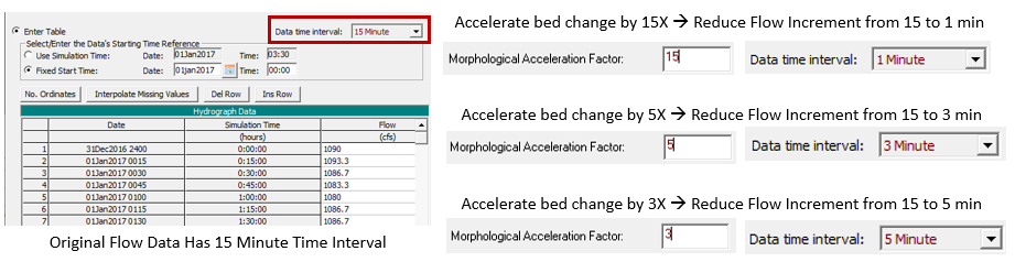

The Morphologic Acceleration Factor should be used with caution as it can lead to misleading results or instabilities. The best practice for using the factor is to test the validity of the factor by doing a full or partial length of a simulation with the factor and without it and compare the results. If the results agree reasonably well, then longer or alterative simulations can usually be done with the Morphologic Acceleration Factor, saving time. It is generally not recommended to use a factor larger than 30 to 50, and values between but not equal to 0 and 1. 

Since, the Morphologic Acceleration Factor is applied to the bed exchange rates, the approach does not change total-load transport rates or concentrations. In addition, the approach is not locally mass conservative but approximately globally conservative.

Finally, it is important to emphasis that the Morphologic Acceleration Factor should NOT be used as a calibration parameter. It should be used carefully and validated to make sure the results are not sensitive to the Morphologic Acceleration Factor. When used carefully the Morphologic Acceleration Factor can be a powerful and useful tool in numerical studies.

Fixed Bed Modeling with the Morphological Acceleration Factor

The Morphologic Acceleration Factor can be utilized in several ways. It used to be the best way to develop a fixed bed sediment model.  Morph Acceleration = 0 ignores bed change but still routes the sediment concentrations. The "Concentration Only" computational mode provides the same capability now, however, and is a more direct method for fixed-bed sediment modeling.

Base Bed-Slope Coefficient

The Base Bed-Slope Coefficient specifies the maximum value of the bed-slope coefficient. The coefficient is then reduced based on the skin and critical shear stresses. As the ratio between the skin and critical shear stress increases bed-load particles are less influenced by the bed slope. The coefficient is used to compute an additional sediment flux in the downslope direction which is a function of the bed slope, the bedload, and the bed-slope coefficient. For further details on the formulation, the user is referred to the HEC-RAS 2D Sediment Technical Reference manual (HEC 2020). The Base Bed-Slope Coefficient typically has a value between 0.1 and 1. Increasing the coefficient has the effect of smoothing the bathymetry. Measured bed change can be used to calibrate the base bed-slope coefficient. However, its effect is significantly less than the transport formula, transport scaling factors and mobility scaling factor. The Base Bed-Slope Coefficient will tend to improve model stability by smoothing out small scale instabilities. However, if the value is too large the numerical scheme can become unstable. In these situations the user can either reduce the computational time step or reduce the value of the Base Bed-Slope Coefficient.

Modeling Note: Base Bed-Slope Coefficient Range

The Base Bed-Slope Coefficient generally varies from 0.1 to 0.5 and higher values tend to smooth results.

Suspended Fraction Equation

In HEC-RAS Version 6.6, the option was added to select a method to component the fraction of suspended sediments. The three methods available are Van Rijn (1984), Greimann et al. (2008), and Jones and Lick (2001). The equation is only used when a transport function is selected which does not already provide an estimate of the equilibrium suspended load fraction. HEC-RAS 2D sediment is a total-load sediment model and the fraction of suspended sediment is separate the total-load into it's bed and suspended components which are used in various calculations. 

Figure 4. 2D Suspended Fraction Equation options in the 2D Sediment Options editor.

Hindered Settling

Hindered settling is the condition in which the settling velocity of particles or flocs is reduced due to a high concentration of particles. Hindered settling is primarily produced by particle collisions and the upward water flow equal to the downward sediment volume flux. Hindered settling occurs to both cohesive and noncohesive particles. However, the hindered settling correction described here only applies to noncohesive particles. The hindered settling of cohesive particles is accounted for in the floc settling method. Currently, the 2D sediment has the option to use the Richardson and Zaki (1954) formula for hindered settling (see figure below). For simplicity the exponent in the Richardson and Zaki (1954) is set to 4.0 and cannot be modified in the user interface.

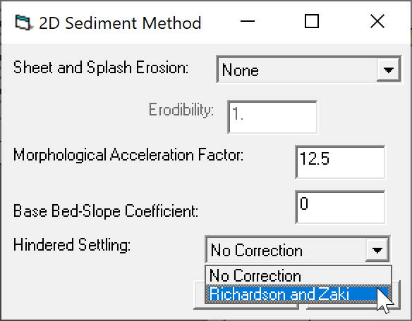
Figure 5. Setting the hindered settling method to the Richardson and Zaki (1954) method.

The figure below shows the ratio of the hindered settling velocity $//<![CDATA[ \begin{array}{l}\omega_{sd}\end{array} //]]>$ and free settling velocity $//<![CDATA[ \begin{array}{l}\omega_{sd0}\end{array} //]]>$ as a function of the total sediment concentration by volume following Richardson and Zaki (1954).

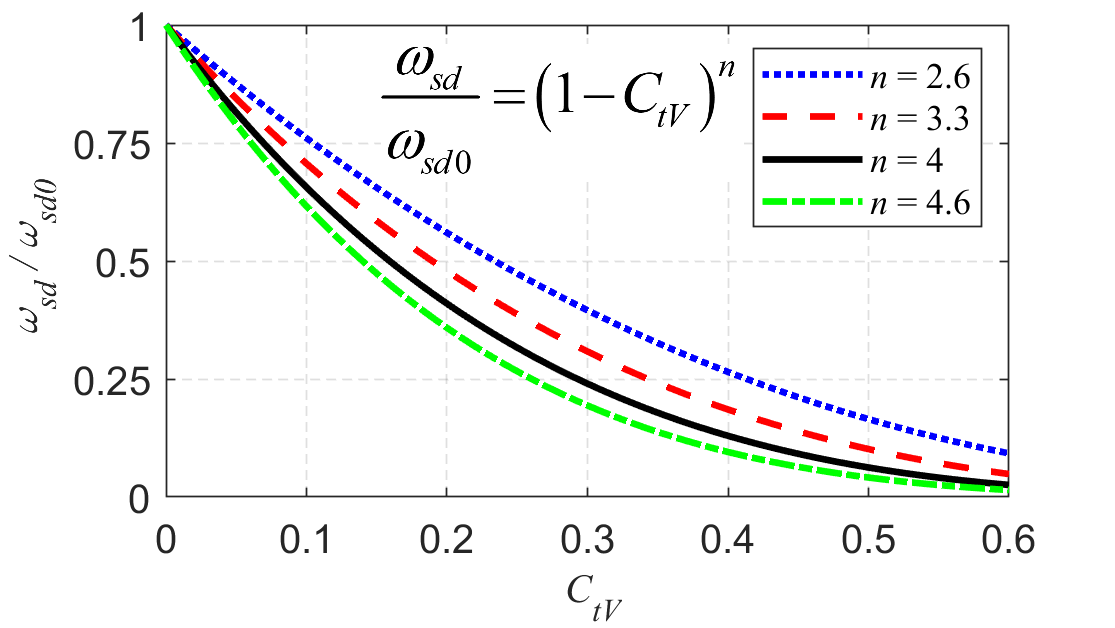
Figure 6. Richardson and Zaki (1954) hindered settling velocity formula.

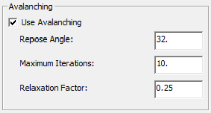
Avalanching

HEC-RAS Version 6.2 and newer support the option to simulate sediment sliding or avalanching. This option limits the bed slope to the angle of repose. A single angle of repose is utilized for both wet and dry cells. The angle of repose can vary from about 30º to nearly vertical for cohesive beds. Avalanching is computed with an iterative relaxation approach which has two parameters: (1) the maximum number of iterations, and (2) a relaxation factor. The recommended range for the maximum number of iterations is between 5 to 20. The range for the relaxation parameter is typically between 0.1 and 0.3. The angle of repose, maximum number of iterations, and relaxation factor are specified in the Avalanching section of the 2D Options menu.