Download PDF
Download page Sediment Boundary Conditions.
Sediment Boundary Conditions
The second tab on the Sediment Data editor defines sediment boundary conditions (see figure below). The editor automatically lists external model boundaries. HEC-RAS requires a boundary condition at all external boundaries. If any external boundary (i.e. boundary condition line) is left unspecified, then an equilibrium sediment load boundary condition is assumed. The types of boundary conditions which may be specified in a 2D sediment model are:
- Rating curve
- Sediment load series
- Equilibrium load
- Clear water (no sediment)
- Capacity Ratio
The other boundary condition options available from the interface (which are mostly associated with 1D flow splits) are not allowed at 2D sediment transport boundaries. Only inflow sediment boundary conditions are required. When the model computes flow out of the domain the sediment can simply leave the domain. At 2D boundaries that where flux is always out of the domain, users can select the equilibrium boundary condition may or simply leave the sediment boundary condition empty. Any boundary condition lines left empty are assigned an Equilibrium Load boundary condition.
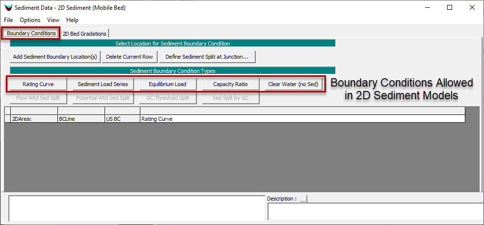
Boundary Conditions tab in the Sediment Data editor.
Downstream Boundary Conditions
Recent versions of HEC-RAS populate boundary conditions for downstream boundary conditions. Two-dimensional models do not recognize "upstream" and "downstream." But earlier versions recognized stage boundary conditions as downstream boundaries and did not populate a sediment boundary condition. Therefore, models that were developed in earlier versions will populate these as blank boundary conditions. It is ok to leave them blank. Blank boundary conditions assume equilibrium sediment boundary conditions. As long flux at these boundaries leaves the model, no sediment boundary condition is applied. However, if flow reverses and flux enters the model at the stage boundary condition, it needs a sediment boundary specification. Users can leave these blank for equilibrium, select equilibrium, take control of the reverse flow sediment load with a rating curve or time series, or keep reverse flow inflows clear with a clear water boundary condition.
Rating Curve
The rating curve specifies the sediment load in tons/day or sediment concentration in mg/l as a function of flow discharge in the first two rows. Users also must specify the percentage of those loads/concentrations that are associated with each grain class in the next 20 rows. HEC-RAS then uses the grain class percentages to compute the sediment flux at the boundary for each size.
Even though the Number of flow-load points dropdown box allows users to add up to 20 columns, users should use the fewest possible flow-load pairs to define their rating curve (preferably 2, but no more than 3-5 if the rating curve is bent or has multiple, clear, grain size transitions).
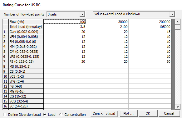
Sediment Rating Curve editor.
Modeling Note: Developing a Flow-Load Rating Curve
This flow-load or flow-concentration rating curve has the same form as the 1D sediment rating curve boundary condition. That part of the user documentation has much more detail on how to develop these data. See Creating a Sediment Rating Curve (Best Practices) for some information on how to develop a sediment rating curve. HEC-RAS also includes a tool that can help users compute a rating curve from flow-load or flow-concentration data (and can even download those data directly from a USGS gage in the United States). See Sediment Rating Curve Analysis Tool to learn how to use that tool.
Using Compound Boundary Conditions (Rating Curve + Equilibrium)
It can be advantageous to use different sediment load boundary conditions for different transport mechanisms. In particular, it is often useful to specify wash load or suspended load, but use equilibrium load for bed load. In previous versions users had to choose between specifying a flow-load/concentration relationship or selecting equilibrium load. More recent versions allow more flexibility with the drop-down box pictured below.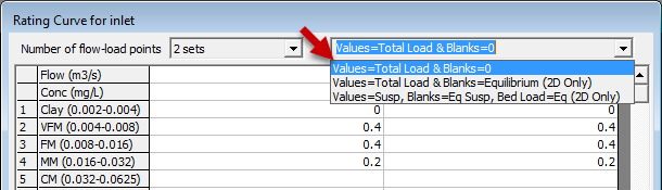
The 2D Sediment Model offers three choices for how to handle blanks and bed load that give users some flexibility:
Method 1: Values = Total Load & Blanks = 0
This is the default method. If this first method is selected, the rating curve boundary condition only uses the specified gradations as total load. It does not make a distinction between bed load and suspended load in the input data (the 2D model does distinguish suspended and bed load in the computations) and blanks in the data grid mean that that grain class is absent at the specified flow.
Method 2: Values = Total Load & Blanks = Equilibrium
In the second method, any data grid cell with a value (e.g. VFM, FM, and MM in the figure above) will use the user specified load in the rating curve. However, if the grain class is blank in the rating curve but is in the bed gradation at the model boundary, HEC-RAS will use the equilibrium load boundary condition for that grain class (i.e. it will compute the capacity to transport the grain class and introduce the mass flux that satisfies that capacity). For now, this is only a 2D method, but this could be introduced to the 1D model as well. It is useful for cases like reservoir or floodplain deposition. Users can specify a fraction of "0" instead of leaving a grain class blank if they do not want the model to introduce any sediment load for that grain class at the boundary condition.
Method 3: Values = Suspended Load & Blanks = Equilibrium Suspended Load, Bed Load Always Uses Equilibrium
The third method computes which grain classes transport by bed load and suspended load for each boundary condition flow. It uses the equilibrium load assumption to compute the boundary condition for grain classes identified as bed load. For grain classes identified as suspended load, it uses the sediment model uses the mass identified in the rating curve editor if the user specifies a mass/fraction for that grain class. Users can force a suspended or wash load grain class to zero by specifying a fraction of "0" (see clay in the example above) instead of leaving it blank.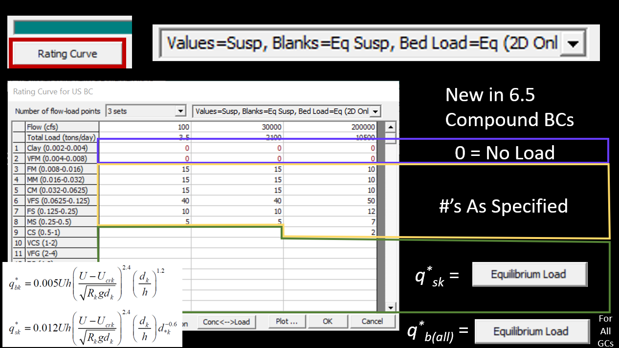
Sediment Load Series
The Sediment Load Series boundary condition specifies the sediment load in tons per time increment (see figure below). The sediment gradation may be specified with a Gradation Rating Curve or if this data is left empty, the gradation is determined by weighting the local (cell) equilibrium sediment loads. The Gradation Rating Curve specifies the gradation of the inflow sediment as a function of total load in tons/day. It is important to keep in mind that any grain specified in the gradation curve is automatically added to the computed grain classes.
Unlike the Rating Curve boundary condition above, the sediment time series editor interpolates the gradation based on the LOAD (in T/d). The sediment load rate in the gradation editor (on the right side of this editor) is in tons per day, while the sediment loads (on the left side of the editor) are just masses spread out over the duration they are associated with. To compute the Total Load Rate, HEC-RAS divides the Sediment Load by the Duration. In the example below the Sediment Loads have a 24 hour duration, so they are input in tonnes/day. But if the duration were shorter or longer, the Sediment Load would not match the Total Load rates for the gradation interpolation.

Sediment Load Series editor.
Equilibrium Load
The Equilibrium Load boundary condition specifies the inflow sediment load as the equilibrium sediment load. The equilibrium sediment load is computed as the equilibrium sediment concentrations at the boundary cells times the face flows. This approximation essentially assumes a zero-gradient concentration normal to the boundary. The equilibrium boundary condition should be used whenever data is not available or when first setting up a model in order to quickly get simulation results or to compare results from other boundary condition types which may be suspect.
Clear Water
The Clear Water boundary condition specifies a zero load/concentration at the boundary. This boundary is not common except for specific situations (e.g. downstream of a high trap efficiency reservoir).
Capacity Ratio
The Capacity Ratio boundary condition specifies a load/concentration at the boundary which is a ratio of the equilibrium load/concentration. This boundary condition is a generalization of the equilibrium boundary condition and is useful for over-loading or under-loading a boundary when there is not much sediment data available. For example, 1.1 will bring in 110% of equilibrium load, which should deposit, and 0.9 will bring into 90% of equilibrium and should erode.
Unsteady Temperature
Temperature is the only data the unsteady flow editor required for sediment transport analyses. Specify temperature for an unsteady sediment transport model in the Unsteady Flow Editor. Select the Water Temperature (for Unsteady Sediment)… option from the Options menu (see figure below).
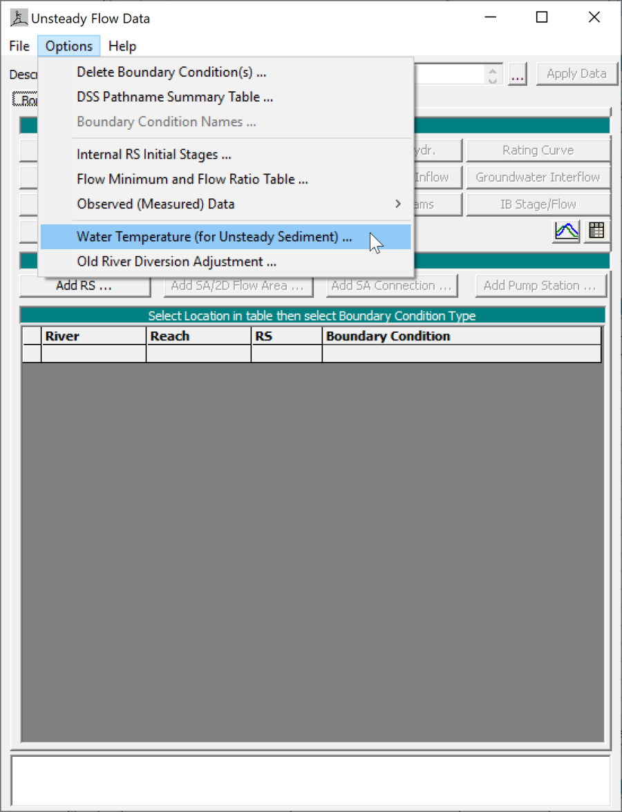
Figure 4. Opening the Unsteady Temperature editor from the Unsteady Flow Data editor.
The Unsteady Temperature time series editor, is similar to the unsteady flow and stage editors (see figure below). In the absence of temperature data in the unsteady flow file, HEC-RAS will assume 55.4ºF. The water temperature is used to compute the water kinematic and dynamic viscosities, and the water density which are then used by the sediment transport model.
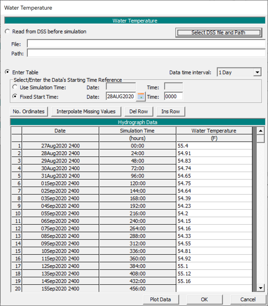
Figure 5. Specifying a temperature time series.