Creating a Sediment Rating Curve (Best Practices)

HEC-RAS Includes a New Tool to Support These Analyses

Since version 6.2, HEC-RAS includes a Sediment Rating Curve Analysis Tool, that downloads or imports sediment data (automatically from a USGS gage) and walks users through the analyses described on this page and video.

Flow load data, if available, are usually noisy, spanning one or two orders of magnitude. Seasonal effects, non-stationarity, hysteresis, sample error and random processes make flow an imperfect predictor of load. Therefore, defining a single flow-load rating curve requires approximating the 'data cloud' with a single curve of flow-load points. Several considerations should guide flow-load estimation.  Best practices in developing a sediment rating curve are discussed below, and several of them are described in the second half of this video:

Gray and Simoes also wrote an excellent chapter in the ASCE Sediment Engineering Manual of Practice (110) on sediment load and rating curve data that provides good context for developing a rating curve boundary condition.

1. Consider Unmeasured Load:
   Most sediment load measurements exclude bed load and near-bed, high concentration suspended load. If the river has substantial bed load, particularly at high flows, augment the flow-load curve to reflect these.
   
   
2. Use Predictor-Correctors to Un-bias Flow-Load Rating Curves:
   The most common way to fit a noisy data cloud, with a general, linear trend in log-log space, is a transformed regression. When Excel or R fit a power function to flow-load data, they log transform the data and then fit a straight line to the log-transformed data with a least-root-mean-squared (LMRE) regression.
   
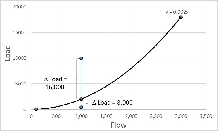
   However, when the regression is untransformed, the positive residuals are always larger than the negative residuals. The figure below shows equal log transformed residuals, that balance in a transformed, LRME, regression (left). But after the reverse transform, the positive residual is almost twice the negative residual. This asymmetry of the transformed residuals biases power fits low. A standard power fit of flow-load data in Excel will underestimate load substantially (often by 5-60%).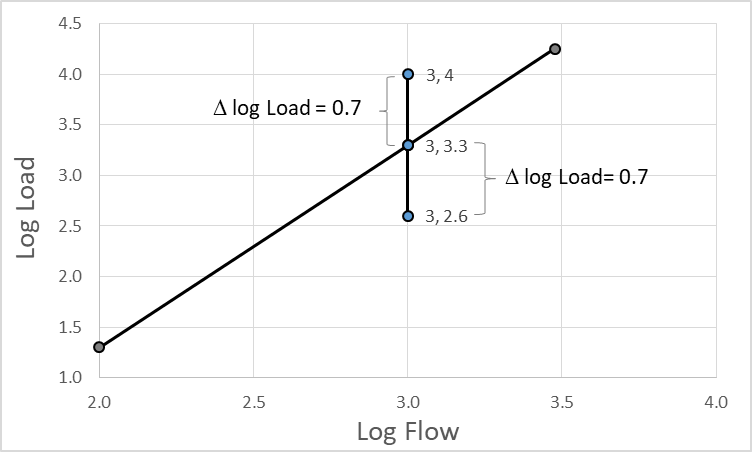
   
   Modelers should unbias their rating curve when fitting a power function to flow-load data. USACE modelers (Copeland and Lombard, 2009) have used Ferguson (1986) correct the transform bias in a flow-load power function. More recently, the USBR, USGS, and USACE modelers tend to use the Duan (1983) 'smearing factor.'*  HEC is working on a Rating Curve calculator to help with this analysis (and others described in this section). At the least, be prepared to increase the loads by 10-60% during model calibration when using an un-corrected, power fit to represent measured flow-load data.  (*Note: Another option is to regress concentration - which is not monotonic - with a polynomial).
3. Select as Few Flow Load Points as Possible:

   A flow-load curve should span the entire range of flows, including a minimum of two points.  The rating curve must include  a low flow and a high flow that bound observed or expected flows and their accompanying loads. A common error involves developing a flow-load rating curve that only extends to the maximum flow with a concentration sample, and not the maximum flow in the model. 
   
   Keep boundary conditions as simple as possible, but no simpler. There are two reasons to add intermediate flow-load points:

   • Rating Curve Slope Change: HEC-RAS uses log interpolation to associate loads with flows between specified flow-load pairs. Sometimes sediment load curves have inflection points, though. Supply limitation may flatten the upper portion of the curve or the curve might steepen in the higher flows. Add intermediate points to capture these inflection points. (below).
     HEC has developed an algorithm to find the inflection point in a rating curve and fit a continuous piecewise-linear regression to a "bent" rating curve.  This will be available in the Rating Curve Analysis tool in future versions of HEC-RAS.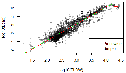
   • Gradation Change: Users must enter gradational breakdowns for each point on the flow-load curve (see Flow-Gradation section). However, gradational changes also require flow-load records. Define intermediate flow-load points at any flow that requires unique gradation data, even if it approximates the load that the rating curve would select automatically.
     
     
4. Calibration:
   Sediment models must be calibrated to provide reliable predictive results. Calibration parameters, those adjusted to replicate historical bed change, should be those that are most uncertain and most sensitive. Sediment models are often highly sensitive to the load boundary condition, which is uncertain even if good data are available. Therefore, estimated flow-load curves should be provisional, refined during the calibration process.
   
   
5. Stationarity Analysis
   Sediment load changes over time. Agricultural impacts, land use changes, fires, mass wasting events, dam removals, and eruptions while dams, pavement, and improved agricultural practices can decrease sediment loads (Walling and Fang (2003).Walling D.E. and Fang D. (2003) "Recent trends in the suspended sediment loads of the world's rivers." Global and Planetary Change 39:111–126.
   
   Because sediment load data are often scarce, modelers want to make use of all the data available. But it is important to test the load stationarity (does it change over time). Plot and analyze the data in time blocks, particularly before and after know system changes like a dam or gravel mining policies. If there is a big shift in the rating curve over time, consider using the most recent data to develop the future conditions rating curve. The effects of climate change on future sediment loads is regional and uncertain. But those considerations can be part of a stationarity analysis as well.
6. Serial Correlation
   Regression analyses – including the transformed, LMSE regression used to fit a power function and unbiasing corrections – assume observation independence. However, most sediment load data are opportunistic. It is common to find several of the load measurements in the flow-load measurements at a gage are collected on the same day.
   
   When developing a flow-load curve, the analyst must decide if these same-day samples are replicates or independent enough to add value. Including replicates, over-weights those observation in the regression and biases the sample (i.e. serial correlation or autocorrelation).
   
   But if the rate-of-rise of the hydrograph is sufficient, these samples can be independent enough to include several or all of them, particularly when they represent and under-sampled portion of the curve (e.g. high, 07Oct2010 flows in Figure 1 59). Figure 1 58 and Figure 1 59 include two examples of flow-load data with same-day sample clusters. However, each sampling day in Figure 1 58 covers a constrained flow range, making these more like replicates. The 07Oct2010 samples in Figure 1 59, however, cover a wide range of flows.
   Modelers should – at least - make this decision, whether to include temporally clustered data as independent observations or average them as replicates. But the best practice includes a statistical test to determine the independence of these data. The USGS software package SAID (The Surrogate Analysis and Index Developer Tool) includes serial correlation analyses and quantitative methods to distinguish observations from replicates.
   
   
7. Statistical Power of Low Flow Samples:
   Most sediment samples are collected at low flows when sampling conditions are safe. However, these loads are not very important morphologically. So many rating curve regressions over-weight the influence of the least significant samples. Use common sense to evaluate the rating curve, recognizing that the 50% recurrence-interval flow (and larger events) will do most of the morphological work in the system. If a quantitative fit of the available data does not reflect the flow-load relationship of the most morphologically significant flows and loads, an estimated hand fit (and using load as a calibration parameter) might be more appropriate.