The example dataset provided is for demonstration purposes only and should not be used for other purposes. Some of the data within the dataset may have been altered specifically for the purpose of testing and demonstration and do not reflect actual conditions at the location. The example model has been simplified where possible for storage size and computation runtime purposes, and is not reflective of detailed study models.
Download: BeaverLake-SWMM-Import-Solution.zip
This example dataset is a catchment area for a neighborhood near Nashville, TN. The model geometry contains a 2D area to which rainfall is applied, and contains a small Pipe Network that drains a portion of the catchment to a downstream lake. This dataset was created by importing the pipe geometry from an EPA SWMM model using the SWMM import tool, and integrating it with a 2D Area. For a step-by-step walkthrough of how to create this dataset, see the Tutorial.
The 2D mesh was refined using breaklines and refinement regions to capture the flow direction of the streets, and to capture controlling elevations in the terrain. The downstream boundary for the 2D area is at the edge of the lake and is set to normal depth, allowing surface water that is not capture by the Pipe Network to leave the model. 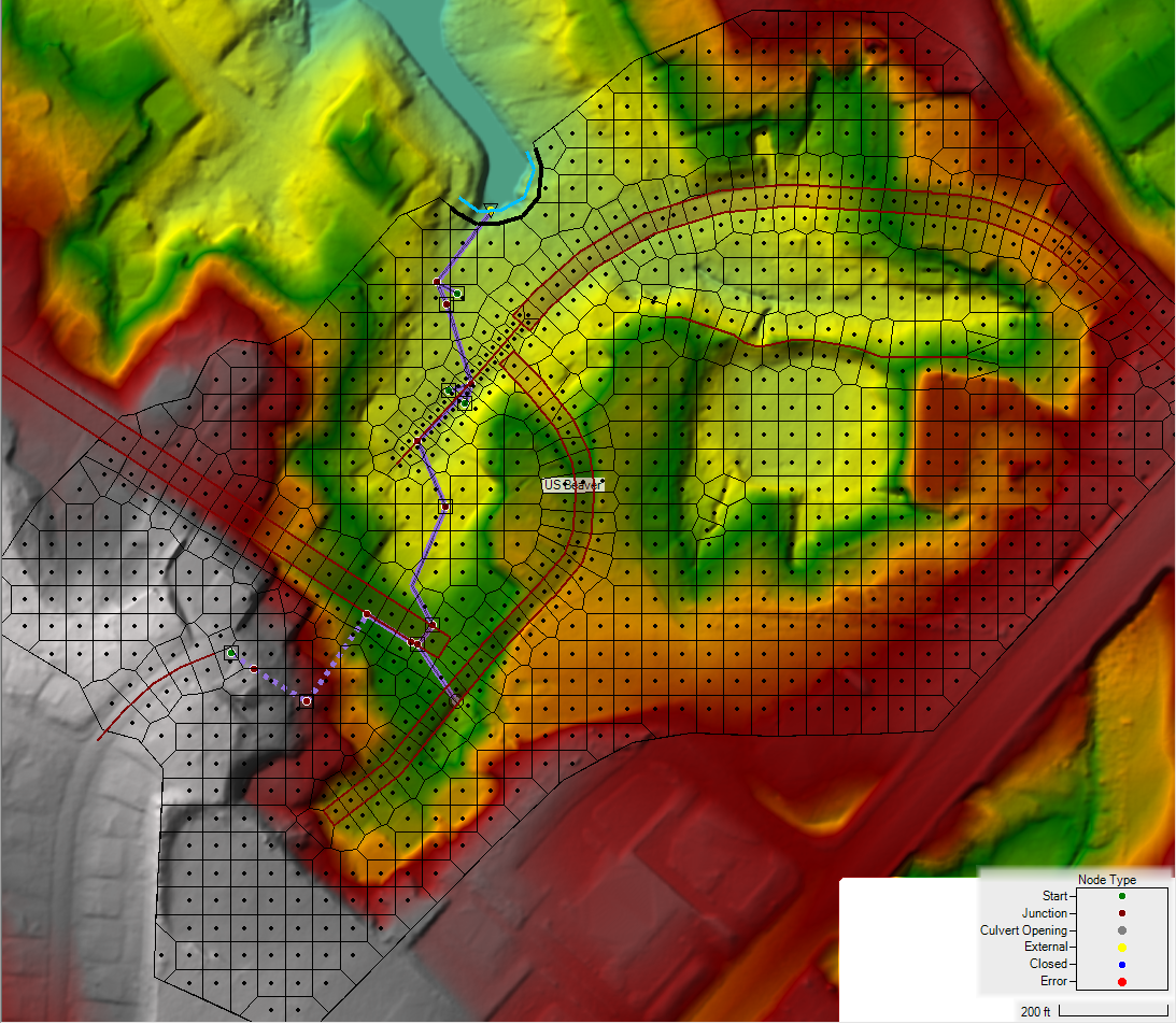
The catchment has some some steeper terrain, (~20% slopes) between terraces so the Pipe Network also contains conduits that are on the steeper side. The steep sloped conduits can require a much smaller timestep and increase the computation time. To avoid those issues, the steep conduits' Computation Method attributes were set to Instantaneous. The Instantaneous method simply transfers inflow from one end of the conduit to the other end without modeling it hydraulically. This allows the inflow from the drop inlets to enter the pipe system without hydraulic routing through the conduits themselves.

Another unique aspect about this dataset is it's small size with about 75 computational cells for the Pipe Network and less than 1000 computational cells for the 2D Area. With such a small Pipe Network, the computational burden of splitting up the problem to run on multiple CPUs is more intensive than the hydraulic computations themselves. That said this dataset sees computational speed benefits by setting the Solver Core Computation Option to just a single core for both the Pipe Network and 2D computational settings.

The steepness of this system is such that, when free flowing, the conduits are all in supercritical flow. But about 1/4 way into the simulation, the system becomes overwhelmed on the downstream end and begins to pressurize the system further upstream. As the system begins surcharging, you can see the HGL increase, and the velocities decrease significantly.

