Download PDF
Download page Estimating Breach Parameters.
Estimating Breach Parameters
The estimation of the breach location, size, and development time are crucial in order to make an accurate estimate of the outflow hydrographs and downstream inundation. However, these parameters are some of the most uncertain in the entire analysis. The HEC-RAS software requires the user to enter the following information to describe a dam breach:
Failure Location: centerline stationing of the breach in the dam
Failure Mode: overtopping or piping
Shape: bottom elevation, bottom width, left and right side slopes H:V
Time: critical breach development time
Trigger Mechanism: pool elevation, pool elevation + duration, or clock time
Weir and Piping Coefficients: weir coefficients are used to compute overtopping/weir flow, and an orifice coefficient is used to compute piping/pressure flow.
Failure Location: The breach failure location is based on many factors (type and shape of dam, failure type, mode, and driving force of the failure). In general, one should consider all factors about the dam, including any historical knowledge of seepage and foundation problems, and place the breach location in the most probable location for each failure type. The geotechnical engineer should be involved in determining the appropriate placement of the breach.
Failure Mode: While HEC-RAS hydraulic computations are limited to overtopping and piping failure modes, all of the other failure modes can still be simulated with one of these two methods. The failure mode is the mechanism for starting and growing the breach. Overtopping failures start at the top of the dam and grow to maximum extents, while a piping failure mode can start at any elevation/location and grow to the maximum extents. The ultimate breach size and breach formation time are much more critical in the estimation of the outflow hydrograph, than the actual failure initiation mode.
Critical Breach Development Time: HEC-RAS requires the user to enter what is called the "critical breach development time." The critical breach development time for HEC-RAS can be described as follows:
Overtopping Failure: The HEC-RAS breach start time is considered to be when the erosion process has migrated to the upstream face of the dam (this is the start of a breach for HEC-RAS). This is the point at which the outflow from the dam will start to increase due to the breach. This condition is depicted in C through D of the figures below. The end of the breach development time for HEC-RAS is when the breach is fully formed and significant erosion has stopped (Figure E below). The breach development ending time should not include the time to completely drain the reservoir pool.
Piping Failure: The HEC-RAS breach starting time for a piping failure is considered to be when a significant amount of flow and material are coming out of the piping failure hole. The breach ending time is considered to be when the breach is, for the most part, fully formed (significant erosion has stopped, not the time until the reservoir pool is emptied).
The estimation of the critical breach development time must be done outside of the HEC-RAS software and entered as input data. Descriptions on how to estimate this time are given below.
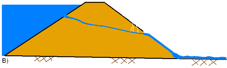
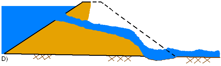
Breach Weir and Piping Flow Coefficients: Weir and piping coefficients must be entered by the user in HEC-RAS. These coefficients directly affect the magnitude of the peak outflow hydrograph for any given breach. Unfortunately, exact knowledge of the magnitude of these coefficients for a dam failure (overtopping or piping failure) is not known. In order to estimate the weir and piping flow coefficients, it is necessary to understand the basic failure process. The following is a generalized description of the breach process for an overtopping failure of an earthen dam. This description may not be true for all earthen dams, as the breach process is a function of many parameters, such as: height of the dam; volume of water behind the dam (including the inflowing hydrograph); materials that the dam is constructed of; depth and duration of overtopping; outer protective cover on the downstream and upstream side of the embankment; etc…
In general, during an overtopping failure of an earthen dam, a headcut erosion process will first start on the downstream side of the dam embankment (see figure A below). While water is going over the dam crest, the dam crest acts like a broad-crested weir. The headcut will erode back towards the center of the dam and widen over time (see figure B below). As the headcut begins to cut into the dam crest, the weir crest length will become shorter, and the appropriate weir coefficient will trend towards a sharp-crested weir value (see figure C below). The time for breach initiation used in HEC-RAS is shortly after what is depicted in figure C below. When the headcut reaches the upstream side of the dam crest, a mass failure of the upstream crest may occur, and the hydraulic control section will act very much like a sharp-crested weir (see figure D below). The headcut will continue to erode upstream through the dam embankment, as well as erode down through the dam and widen at the same time (see figure E below). During this process, the appropriate weir coefficient will begin to trend back towards a broad-crested weir coefficient. As the downward cut reaches the natural river bed elevation, and the breach is more in a widening phase, the appropriate weir coefficient is more in the range of a broad-crested weir value.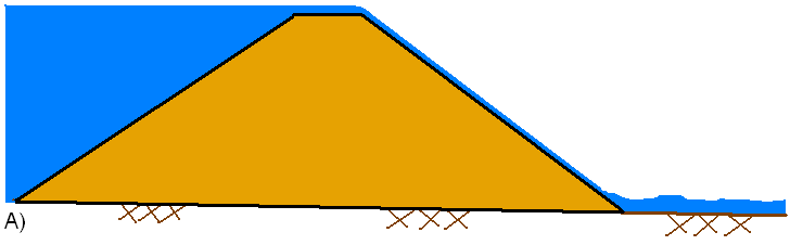
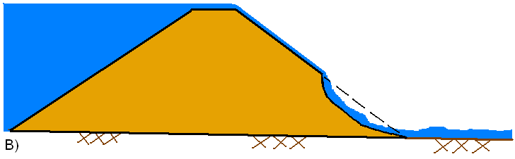
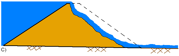
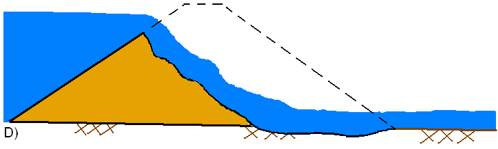

A general description of a piping failure is as follows. Water is seeping through the dam at a significant enough rate, such that it is internally eroding material and transporting it out of the dam. As the material is eroded, a larger hole is formed, thus able to carry more water and erode more material (see figure A below). The movement of water through the dam during this process is modeled as a pressurized orifice type of flow. During the piping flow process, erosion and headcutting will begin to occur on the downstream side of the dam (see figure B below) as a result of flow exiting the pipe. As the piping hole grows larger, material above the hole will begin to slough off and fall into the moving water (see figure C below). The headcutting and material sloughing processes will continue to move back towards the upstream side of the dam, while the piping hole continues to grow simultaneously (see figure D below). If the piping hole is large enough, the weight of the material above the hole may be too great to be maintained, and a mass caving of material will occur. This will result in a large rise in the outflow through the breach and will accelerate the breaching process. Also at this point, the hydraulics of the flow transitions from a pressure/orifice type flow to an open air weir type flow. The headcutting and erosion process then continues back through the dam, as well as downward (see figure E below). Additionally, the breach will be widening. Depending on the volume of water behind the dam, the breach may continue to cut down and widen until the natural channel bed is reached. Then the breach will go into a widening phase. 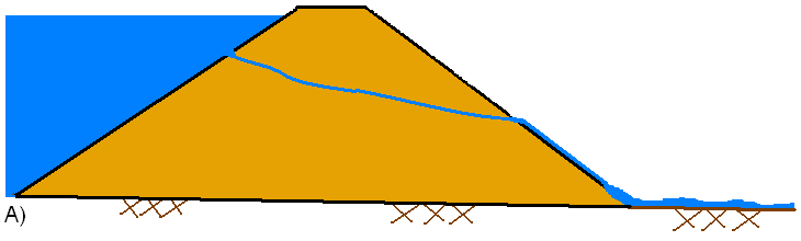


As you can imagine from the description of the breach processes described above, as well as other factors and complications that may occur in the real world, estimating these parameters can be difficult. Currently in computer programs such as HEC-RAS, the user is only allowed to enter a single value for the breach weir coefficient and for the piping coefficient. Because the estimate of the peak flow is so important in this process, one should try to estimate these coefficients based on the phase of the breach process in which they think the largest flows will most likely occur. For example, earthen dams with medium to very large storage volumes upstream, will most likely have failed all the way down to the natural stream bed elevation, and be in the breach widening phase when the peak outflow occurs. This would suggest using a weir coefficient that is typical of a broad-crested weir with a long crest length (i.e. C = 2.6). However, for dams with a relatively low volume of water in comparison to the height of the dam, the peak flow may occur during the phase of the breach in which the breach is still cutting down through the dam. For this case, a weir coefficient typical of a sharp-crested weir would be more appropriate (i.e. C = 3.2). Other factors to consider are the material types of the dam. Dams that have a clay core, and are generally constructed of clay material, will tend to have a much more pronounced headcut process. While dams that are more in the sand and gravel range will have a less pronounced headcut process. This may lead to using higher weir coefficients for a clay dam (i.e. C=3.2, sharp-crested weir) versus a gravel/sand dam (i.e. C=2.6, broad-crested weir).
During a piping failure breach, the rate of water flowing through the dam is modeled with an orifice pressure flow equation. This equation also requires a discharge coefficient, which is a measure of how efficiently the flow can get into the pipe orifice. Because a piping failure is not a hydraulically designed opening, it is assumed that the entrance is not very efficient. Recommended values for the piping/pressure flow coefficients are in the range of 0.5 to 0.6.
Guidelines for selecting breach weir and piping flow coefficients are provided in the table below.
Dam breach weir and piping coefficients
Dam Type | Overflow/Weir | Piping/Pressure Flow |
|---|---|---|
Earthen Clay or Clay Core | 2.6 – 3.3 | 0.5 – 0.6 |
Earthen Sand and gravel | 2.6 – 3.0 | 0.5 – 0.6 |
Concrete Arch | 3.1 – 3.3 | 0.5 – 0.6 |
Concrete Gravity | 2.6 – 3.0 | 0.5 – 0.6 |
Breach Shape Definitions. For the purposes of these guidelines, the physical description of the breach will consist of the height of the breach, breach width, and side slopes in H:V. These values represent the maximum breach size. A diagram describing the breach is shown in the figure below.

The breach width is described as the average breach width (Bave) in many equations, while HEC-RAS requires the breach bottom width (Wb) for input. The breach height (hb) is the vertical extent from the top of the dam to the average invert elevation of the breach. Many publications and equations also use the height of the water (hw), which is the vertical extent from the maximum water surface to the invert elevation of the breach. The side slopes are expressed in units of distance horizontal to every one unit in the vertical (H: 1V).
The breach dimensions, as well as the breach formation time must be estimated outside of the HEC-RAS software, and entered into the program. Many case studies have been performed on data from historic dam failures, leading to guidelines, regression equations, and computer modeling methodologies for prediction of the dam breach size and time. One of the most comprehensive summaries of the literature on historic dam failures is a Bureau of Reclamation report written by Tony Wahl titled "Prediction of Embankment Dam Breach Parameters" (Wahl, 1998). This report discusses all types of dams, however it focuses on earthen/embankment dams for the discussion of estimating breach parameters. Much of what is presented in this section was extracted from that report. Guidelines for breach parameters for concrete (arch, gravity, buttress, etc), steel, timber, and other types of structures, are very sparse, and are limited to simple ranges.
Federal Agency Guidelines. Many federal agencies have published guidelines in the form of possible ranges of values for breach width, side slopes, and development time. Table 14-3 below summarizes some of these guidelines.
Table 13-3. Ranges of possible values for breach characteristics.
Dam Type | Average | Horizontal | Failure Time | Agency |
|---|---|---|---|---|
Earthen/ | (0.5 to 3.0) x HD | 0 to 1.0 | 0.5 to 4.0 | COE 1980 |
Concrete | Multiple Monoliths | Vertical | 0.1 to 0.5 | COE 1980 |
Concrete | Entire Dam | Valley wall slope | ≤ 0.1 | COE 1980 |
Slag/ | (0.8 x L) to L | 1.0 to 2.0 | 0.1 to 0.3 | FERC |
Where:
HD = Height of the Dam.
L = Length of the Dam crest.
*Note: Dams that have very large volumes of water, and have long dam crest lengths, will continue to erode for long durations (i.e. as long as a significant amount of water is flowing through the breach), and may therefore have longer breach widths and times than what is shown in Table 14-3.
The guidelines shown in Table 14-3 should be used as minimum and maximum bounds for estimating breach parameters. More specific ways to estimate breach characteristics are addressed below.
Regression Equations. Several researchers have developed regression equations for the dimensions of the breach (width, side slopes, volume eroded, etc…), as well as the failure time. These equations were derived from data for earthen, earthen with impervious core (i.e. clay, concrete, etc…), and rockfill dams, and therefore do not directly apply to concrete dams or earthen dams with concrete cores. The report by Wahl (1998) describes several equations that can be used for estimating breach parameters. Summarized in the figure below are the regression equations developed to predict breach dimensions and failure time from the USBR report (Wahl, 1998). .")
Since the report by Wahl, additional regression equations have been developed to estimate breach width and breach development time. In general, several of the regression equations should be used to make estimates of the breach dimensions and failure time. These estimates should then be used to perform a sensitivity analysis, as discussed later in this chapter. The user should try to pick regression equations that were developed with data that is representative of the study dam. In many cases this may not be possible, due to the fact that most of the historic dam failures for earthen dams have occurred on smaller structures. In fact, out of the 108 historic dam breaches listed in the USBR report (Wahl, 1998), only 13 of the dams are over 100 ft (30.5 m) high and only 5 of the dams had a storage volume greater than 100,000 acre-feet (123.4x10⁶ m3) at the time of failure. Additionally, most of the regression equations were developed from a smaller subset of this data (20 to 50 dams), and the dams included in the analysis are a mixture of homogenous earthen dams and zoned earthen dams (dams with clay cores, or varying materials). Therefore, the use of any of the regression equations should be done with caution, especially when applying them to larger dams that are outside the range of data for which the equations were developed. The use of regression equations for situations outside of the range of the data they for which were developed for may lead to unrealistic breach dimensions and development times.
The following regression equations have been used for several dam safety studies found in the literature (except the Xu and Zhang equations, which are presented because of their wide range of historical data values), and are presented in greater detail in this chapter:
- Froehlich (1995a)
- Froehlich (2008)
- MacDonald and Langridge-Monopolis (1984)
- Von Thun and Gillette (1990)
- Xu and Zhang (2009)
These regression equations have been used on several dam break studies and have been found to give a reasonable range of values for earthen, zoned earthen, earthen with a core wall (i.e. clay), and rockfill dams. The following is a brief discussion of each equation set.
Froehlich (1995a):
Froehlich utilized 63 earthen, zoned earthen, earthen with a core wall (i.e. clay), and rockfill data sets to develop a set of equations to predict average breach width, side slopes, and failure time. The data that Froehlich used for his regression analysis had the following ranges:
Height of the dams: 3.66 – 92.96 m (12 – 305 ft) with 90% < 30 m, and 76% < 15 m
Volume of water at breach time: 0.0130 – 660.0 m3 x 106 (11 - 535,000 acre-ft) with 87% < 25.0 m3 x 106, and 76% < 15.0 m3 x 106
Froehlich's regression equations for average breach width and failure time are:
| B_{ave} =0.1803K_0 V^{0.32}_w h^{0.19}_b |
| t_f =0.00254 V^{0.53}_w h^{-0.90}_b |
| Symbol | Description | Units |
|---|---|---|
B_{ave} | Average breach width | m |
K_0 | Constant (1.4 for overtopping failures, 1.0 for piping) | |
V_w | Reservoir volume at time of failure | m3 |
h_b | Height of the final breach | m |
t_f | Breach formation time | hrs |
Froehlich states that the average side slopes should be:
1.4H:1V Overtopping failures
0.9H:1V Otherwise (i.e. piping/seepage)
While not clearly stated in Froehlich's paper, the height of the breach is normally calculated by assuming the breach goes from the top of the dam all the way down to the natural ground elevation at the breach location.
Froehlich (2008):
In 2008 Dr. Froehlich updated his breach equations based on the addition of new data. Dr. Froehlich utilized 74 earthen, zoned earthen, earthen with a core wall (i.e. clay), and rockfill data sets to develop a set of equations to predict average breach width, side slopes, and failure time. The data that Froehlich used for his regression analysis had the following ranges:
Height of the dams: 3.05 – 92.96 m (10 – 305 ft) with 93% < 30 m, and 81% < 15 m
Volume of water at breach time: 0.0139 – 660.0 m3 x 106 ( 11.3 - 535,000 acre-ft) with 86% < 25.0 m3 x 106, and 82% < 15.0 m3 x 106
Froehlich's regression equations for average breach width and failure time are:
| B_{ave} =0.27K_0 V^{0.32}_w h^{0.04}_b |
| t_f =63.2 \sqrt{ \frac{V_w}{gh^2_b}} |
| Symbol | Description | Units |
|---|---|---|
B_{ave} | Average breach width | m |
K_0 | Constant (1.3 for overtopping failures, 1.0 for piping) | |
V_w | Reservoir volume at time of failure | m3 |
h_b | Height of the final breach | m |
g | Gravitational acceleration (9.80665) | m/s2 |
t_f | Breach formation time | sec. |
Froehlich's 2008 paper states that the average side slopes should be:
1.0 H:1V Overtopping failures
0.7 H:1V Otherwise (i.e. piping/seepage)
While not clearly stated in Froehlich's paper, the height of the breach is normally calculated by assuming the breach goes from the top of the dam all the way down to the natural ground elevation at the breach location.
MacDonald and Langridge – Monopolis (1984):
MacDonald and Langridge-Monopolis utilized 42 data sets (predominantly earthfill, earthfill with a clay core, and rockfill) to develop a relationship for what they call the "Breach Formation Factor." The Breach Formation Factor is a product of the volume of water coming out of the dam and the height of water above the dam. They then related the breach formation factor to the volume of material eroded from the dam's embankment. The data that MacDonald and Langridge-Monopolis used for their regression analysis had the following ranges:
Height of the dams: 4.27 – 92.96 m (14 – 305 ft) with 76% < 30 m, and 57% < 15 m
Breach Outflow Volume: 0.0037 – 660.0 m3 x 106 (3 - 535,000 acre-ft) with 79% < 25.0 m3 x 106, and 69% < 15.0 m3 x 106
The following is the MacDonald and Langridge-Monopolis equation for volume of material eroded and breach formation time, as reported by Wahl (1998):
For earthfill dams:
| V_{eroded} =0.0261 (V_{out} \times h_w )^{0.769} |
| t_f = 0.0179 (V_{eroded} )^{0.364} |
For earthfill with clay core or rockfill dams:
| V_{eroded} =0.00348 (V_{out} \times h_w )^{0.852} |
| Symbol | Description | Units |
|---|---|---|
V_{eroded} | Volume of material eroded from the dam embankment | m3 |
V_{out} | Volume of water that passes through the breach. i.e. storage volume at time of breach plus volume of inflow after breach begins, minus any spillway and gate flow after breach begins. | m3 |
h_w | Depth of water above the bottom of the breach | m |
t_f | Breach formation time | hrs |
The V_{out} parameter is not exactly known before performing the breach analysis, as it is the volume of water that passes through the breach (not including flow from gates, spillways, and overtopping of the dam away from the breach area). A good first estimate is the volume of water in the reservoir at the time the breach initiates. Once a set of parameters are estimated, and a breach analysis is performed, the user should go back and try to make a better estimate of the actual volume of water that passes through the breach. Then recalculate the parameters with that volume. The recalculation of the volume makes the method iterative. The actual breach dimensions are a function of the volume eroded. The MacDonald and Langridge-Monopolis paper states that the breach should be trapezoidal with side slopes of 0.5H:1V. The breach size is computed by assuming the breach erodes vertically to the bottom of the dam and it erodes horizontally until the maximum amount of material has been eroded or the abutments of the dam have been reached. The base width of the breach can be computed from the dam geometry with the following equation (State of Washington, 1992):
| \displaystyle W_b = \frac{V_{eroded}-h^2_b (CZ_b +h_b Z_b Z_3 /3)}{h_b (C+h_b Z_3 /2)} |
| Symbol | Description | Units |
|---|---|---|
W_b | Bottom width of the breach | m |
h_b | Height from the top of the dam to bottom of breach | m |
C | Crest width of the top of dam | m |
Z_3 | Z_1 + Z_2 | |
Z_1 | Average slope (Z1:1) of the upstream face of dam. | |
Z_2 | Average slope (Z2:1) of the upstream face of dam. | |
Z_b | Side slopes of the breach (Zb:1), 0.5 for the MacDonald method. |
Note: The MacDonald and Langridge-Monopolis paper states that the equation for the breach formation time is an envelope of the data from the earthfill dams. An envelope equation implies that the equation will tend to give high estimates (too long) of the actual breach time (for homogenous earthfill dams). Wahl's study states this method will over predict times in some cases, while many equations will under predict.
Von Thun and Gillette (1990):
Von Thun and Gillette used 57 dams from both the Froehlich (1987) paper and the MacDonald and Langridge-Monopolis (1984) paper to develop their methodology. The method proposes to use breach side slopes of 1.0H:1.0V, except for dams with cohesive soils, where side slopes should be on the order of 0.5H:1V to 0.33H:1V. The data that Von Thun and Gillette used for their regression analysis had the following ranges:
Height of the dams: 3.66 – 92.96 m (12 – 305 ft) with 89% < 30 m, and 75% < 15 m
Volume of water at breach time: 0.027 – 660.0 m3 x 106 ( 22 - 535,000 acre-ft) with 89% < 25.0 m3 x 106, and 84% < 15.0 m3 x 106
The Von Thun and Gillette equation for average breach width is:
| B_{ave} =2.5h_w +C_b |
| Symbol | Description | Units |
|---|---|---|
B_{ave} | Average breach width | m |
h_w | Depth of water above the bottom of the breach | m |
C_b | Coefficient, which is a function of reservoir size, see table below. |
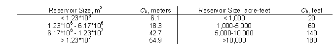
Von Thun and Gillette developed two different sets of equations for the breach development time. The first set of equations shows breach development time as a function of water depth above the breach bottom:
| t_f =0.02 h_w + 0.25 \;(erosion \;resistant) |
| t_f =0.015 h_w \;(easily \;erodible) |
| Symbol | Description | Units |
|---|---|---|
t_f | Breach formation time | hrs |
h_w | Depth of water above the bottom of the breach | m |
The second set of equations shows breach development time as a function of water depth above the bottom of the breach and average breach width:
| \displaystyle t_f = \frac{B_{ave}}{4h_w} \; \;(erosion \;resistant) |
| \displaystyle t_f = \frac{B_{ave}}{4h_w +61.0} \; \;(easily \;erodible) |
Where: B_{ave}=Average breach width (m)
Note that Von Thun and Gillette's breach formation time equations are presented for both "erosion resistant" and "easily erodible" dams. Their paper states: "It is suggested that these limits be viewed as upper and lower bounds corresponding respectively to well-constructed dams of erosion resistant materials and poorly-constructed dams of easily eroded materials".
Xu and Zhang (2009):
In 2009 a paper was published by Y. Xu and L.M. Zhang in the Journal of Geotechnical and Geo-Environmental Engineering. The database gathered by Xu and Zang contained 182 earth and rockfill dams from the United States and China, with nearly 50% of the dams greater than 15 meters in height. However, their final equations are based on a much smaller subset of these dams due to missing data. Their paper shows details for 75 dams that were composed of homogeneous earth fill, zoned-filled, dams with core walls, and concrete faced dams. Their final equation for the average breach width is based on 45 dam failures, and their equation for the time of failure is based on only 28 dam failures.
The data that Xu and Zhang used for their regression analysis had the following ranges:
Height of the dams: 3.2 – 92.96 m (10 – 305 ft) with 78% < 30 m, and 58% < 15 m
Volume of water at breach time: 0.105 – 660.0 m3 x 106 (11.3 - 535,000 acre-ft) with 80% < 25.0 m3 x 106, and 67% < 15.0 m3 x 106
Xu and Zhang's regression equation for average breach width is:
| \displaystyle \frac{B_{ave}}{h_b} =0.787 \left( \frac{h_d}{h_r} \right) ^{0.133} \left( \frac{V^{1/3}_w}{h_w} \right) ^{0.652} e^{B_3} |
| Symbol | Description | Units |
|---|---|---|
B_{ave} | Average breach width | |
V_w | Reservoir volume at time of failure | m3 |
h_b | Height of the final breach | |
h_d | Height of the dam | |
h_r | 15 meters, which is considered to be a reference height for distinguishing large dams from small dams. | |
h_w | Height of the water above the breach bottom elevation at time of breach (m). | |
B_3 | b3+b4+b5 Coefficient that is a function of dam properties | |
b_3 | -0.041, 0.026, and -0.226 for dams with corewalls, concrete faced dams, and homogeneous/zoned-fill dams, respectively. | |
b_4 | 0.149 and -0.389 for overtopping and seepage/piping, respectively. | |
b_5 | 0.291, -0.14, and -0.391 for high, medium, and low dam erodibility, respectively |
The Xu and Zhang paper does not provide estimates for side slopes directly. Instead, they provide an equation to estimate the Top Width of the breach, which can then be used with the average breach width, to compute the corresponding side slopes. Here is their equation for the breach top width:
| \displaystyle \frac{B_t}{h_b} =1.062 \left( \frac{h_d}{h_r} \right) ^{0.092} \left( \frac{V^{1/3}_w}{h_w} \right) ^{0.508} e^{B_2} |
| Symbol | Description | Units |
|---|---|---|
B_t | Breach top width | m |
B_2 | b3+b4+b5 Coefficient that's is a function of Dam Properties | |
b_3 | 0.061, 0.088, and -0.089 for dams with corewalls, concrete faced dams, and homogeneous/zoned-fill dams, respectively. | |
b_4 | 0.299 and -0.239 for overtopping and seepage/piping, respectively. | |
b_5 | 0.411, -0.062, and -0.289 for high, medium, and low dam erodibility, respectively |
Breach side slopes can be computed with the following equation:
| \displaystyle Z= \frac{B_t - B_w}{h_b} |
Important Note
The data Xu and Zhang used in the development of the equation for breach development time includes more of the initial erosion period and post erosion period than what is generally used in HEC-RAS for the critical breach development time. In general, this equation will produce breach development times that are greater than the other four equations described above. Because of this fact, the Xu Zhang equation for breach development time should not be used in HEC-RAS. However, it is shown here for completeness of their method:
\displaystyle \frac{T_f}{T_r} =0.304 \left( \frac{h_d}{h_r} \right) ^{0.707} \left( \frac{V^{1/3}_w}{h_w} \right) ^{1.228} e^{B_5}
Where:
T_f =Breach Formation time (hrs)
T_r =1 hour (unit duration)
V_w =Reservoir volume at time of failure (m3)
h_d =Height of the dam (m)
h_r =15 meters, which is considered to be a reference height for distinguishing large dams from small dams.
h_w =Height of the water above the breach bottom elevation at time of breach (m)
B_5 = b3+b4+b5 Coefficient that is a function of dam properties
b_3 =-0.327, -0.674, and -0.189 for dams with corewalls, concrete faced dams, and homogeneous/zoned-fill dams, respectively.
b_4 =-0.579 and -0.611 for overtopping and seepage/piping, respectively.
b_5 =-1.205, -0.564, and 0.579 for high, medium, and low dam erodibility, respectively.
While not clearly stated in the Xu and Zhang paper, the height of the breach is normally calculated by assuming the breach goes from the top of the dam all the way down to the natural ground elevation at the breach location.
Simplified Physical Breaching Method
The Simplified Physical breaching method allows the user to enter velocity versus breach down-cutting and breach widening relationships, which are then used dynamically to figure out the breach progression versus the actual velocity being computed through the breach, on a time step by time step basis. The main data requirement differences between this method and the User Entered Data breach method, are the following:
Max Possible Bottom Width – This field is now used to enter a maximum possible breach bottom width. This does not mean the entered value will be the final breach bottom width; it is really being used to limit the breach bottom width growth to this amount. The actual bottom width will be dependent on the velocity verses erosion rate data entered, and the hydraulics of flow through the breach. This field is used to prevent breaches from growing larger than this user set upper limit during the run.
Min Possible Bottom Elev – This field is used to put a limit on how far down the breach can erode during the breaching process. This value is not necessarily the final breach bottom elevation; it is a user entered limiter (i.e. the breach cannot go below this elevation). The final breach elevation will be dependent on the velocity verses erosion rate data entered, and the hydraulics of flow through the breach.
Starting Notch Width or Initial Piping Diameter – If the Overtopping Failure mode is selected, the user will be asked to enter a starting notch width. The software will use this width at the top of the dam to compute a velocity. From the velocity it will get a down cutting erosion rate (based on user entered data), which will be used to start the erosion process. If a Piping Failure mode is selected, the user must enter an initial piping diameter. Once the breach is triggered to start, this initial hole will show up immediately. A velocity will be computed through it, then the down cutting and widening process will begin based in user entered erosion rate data.
Mass Wasting Feature – This option allows the user to put a hole in the dam or the levee at the beginning of the breach, in a very short amount of time. This option would probably most often be used in a levee evaluation, in which a section of the levee may give way (Mass Wasting), then that initial hole would continue to erode and widen based on the erosion process. The required data for this option is a width for the mass wasting hole; duration in hours that this mass wasting occurs over (this would normally be a short amount of time); and the final bottom elevation of the initial mass wasting hole (It is assumed that the hole is open all the way to the top of the levee or dam if this option is used).
Velocity vs. Downcutting and Widening Erosion Rates. When using the Simplified Physical breaching option, the user is required to enter velocity versus downcutting erosion rates, as well as velocity versus erosion widening rates. An example of the required data input for this method is shown below in the figure below.
As shown in the figure above, the user is required to enter velocity versus downcutting erosion rates and velocity versus erosion widening rates. This data is often very difficult to come by. Users will need to consult with geotechnical engineers to come up with reasonable estimates of this data for their specific levee or dam. Another way to estimate this information is to try to derive it by simulating a historic levee or dam breach, and adjusting the velocity versus erosion rate data until the model simulates the correct breach width and time. This is obviously an iterative process, and may require the user to perform this at multiple locations to see if there is a consistent set of erosion rates that will provide a reasonable model for simulating levee breaches (or dams) in your geographical area. We realize that this data is not readily available for any specific levee or dam. The hope is that over time we will be able to develop guidelines for these erosion rates based on analyzing historical levee and dam breaches. Additionally, users can try to back into a set of erosion rates in order to reproduce historic levee breaches in their area, then use these relationships to analyze potential future levee breaches.
Physically-Based Breach Computer Models. Several computer models have been developed that attempt to model the breach process using sediment transport theories, soil slope stability, and hydraulics. Wahl (1998) summarized some of these models in his report "Prediction of Embankment Dam Breach Parameters." A table from Wahl's (1998) report, which summarizes the physically based computer models he reviewed is shown in Table 14-4 below.
Table 13-4. Physically-based embankment dam breach computer models.
Model and Year | Sediment | Breach | Parameters | Other |
|---|---|---|---|---|
Cristofano (1965) | Empirical | Constant breach | Angle of | |
Harris and Wagner (1967) | Schoklitsch | Parabolic | Breach | |
Lou (1981); | Meyer-Peter | Regime type | Critical shear | Tailwater |
BREACH (Fread, 1988) | Meyer-Peter | Rectangular, | Critical shear, | Tailwater |
BEED (Singh and Scarlatos, 1985) | Einstein- | Rectangular or | Sediment, | Tailwater |
FLOW SIM 1 and FLOW SIM 2 (Bodine, undated) | Linear predetermined | Rectangular, | Breach |
In general, all of the models listed in Table 14-4 rely on the use of bed-load sediment transport equations, which were developed for riverine sediment transport processes. The use of these models should be viewed as an additional way of "estimating" the breach dimensions and breach development time.
Of all the models listed in Table 14-4, the BREACH model developed by Dr. Danny Fread (1988) has been used the most for estimating dam breach parameters. Dr. Fread's model can be used for constructed earthen dams as well as landslide formed dams. The model can handle forming breaches from either overtopping or piping/seepage failure modes. The software uses weir and orifice equations for the hydraulic computation of flow rates. The Meyer-Peter and Muller sediment transport equation is used to compute transport capacity of the breach flow. Breach enlargement is governed by the rate of erosion, as well as the collapse of material from slope failures. The software can handle up to three material layers (inner core, outer portion of the dam, and a thin layer along the downstream face). The material properties that must be described are: internal friction angle; cohesive strength, grain size of the material (D50), unit weight, porosity, ratio of D90 to D30, and Manning's n. This software has been tested on a limited number of data sets, but has produced reasonable results.
Additional research on the erosion process of earthen embankments that are overtopped is being conducted in the US as well as Europe. The Agricultural Research Service (ARS) has been testing earthen embankment failures at sizes ranging from small scale laboratory models to near prototype scale dams (up to 7 ft high) for several years (Hanson, et al. 2003, Hassan, et al. 2004). Similar tests have been performed in Norway for earthen dams, 5 to 6 meters high, constructed of rock, clay, and glacial moraine (Vaskinn, et al., 2004). The hope is that this research work will lead to the development of improved computer models of the breach process. A dam safety interest group made up of US Government agencies (USBR, ARS, USACE), private industry, and Canadian and European research partners is currently evaluating new technologies for simulating the breach process. The goal of this effort is to develop computer simulation programs that can model the dam breach process by progressive erosion for earthen dams initiated by either overtopping flow or seepage. Computer models that are currently being evaluated are: WINDAM (Temple, et. Al. 2006. ); HR-BREACH (Mohammed et. Al., 2002. HR Wallingford); and FIREBIRD (Wang and Kahawita, 2006. Ecole Polytechnique de Montreal, Canada). Table 14-5 below is a summary of these models capabilities (Tony L. Wahl, 2009):
Table 13-5. Summary of Erosion Process Models Currently Under Development.
Model and Year | Embankment Types | Failure Modes | Erosion Processes |
|---|---|---|---|
WINDAM | Homogeneous with varying levels of cohesiveness | Overtopping | Headcut formation on downstream face, deepening, and upstream advancement; lateral widening |
HR-BREACH | Homogeneous cohesive, or simple composite embankments with noncohesive zones, surface protection (grass or rock), and cohesive cores | Overtopping | Variety of sediment transport/erosion equations and multiple methods of application. Discrete breach growth using bending, shear, sliding and overturning failure of soil masses. |
FIREBIRD | Homogeneous cohesive or noncohesive | Overtopping | Coupled equations for hydraulics and sediment transport. |
Peak Flow Equations and Envelope Curves. Several researchers have developed peak flow regression equations from historic dam failure data. The peak flow equations were derived from data for earthen, zoned earthen, earthen with impervious core (i.e. clay, concrete, etc…) and rockfill dams only, and do not apply to concrete dams. In general, the peak flow equations should be used for comparison purposes.
Once a breach hydrograph is computed from HEC-RAS, the computed peak flow from the models can be compared to these regression equations as a test for reasonableness. However, one should use great caution when comparing results from these equations to model predictions. First, the user should go back to the original paper for each equation and evaluate the data sets and assumptions that were used to develop that equation. Many of the equations were developed from limited data sets, and most were for smaller dams. Also, when using these equations to compare against model results, the event being studied can have a significant impact on the model result's peak flow. For example, studies being performed with Probable Maximum Flood (PMF) inflows may have larger computed peak outflows than what will be predicted by some of the peak flow equations. This is due to the fact that none of the historic data sets were experiencing a PMF level flood when they failed.
Shown below is a summary of some of the peak flow equations that have been developed from historic dam failures:
- Bureau of Reclamation (1982):
Q = 19.1(hw)^{1.85} (envelope equation)
- MacDonald and Langridge-Monopolis (1984):
Q=1.154(V_wh_w)^{0.412}
Q=3.85(V_wh_w)^{0.411} (envelope equation)
- Froehlich (1995b):
Q=0.607V_w^{0.295}h_w^{1.24}
- Xu and Zhang (2009):
\displaystyle \frac{Q}{\sqrt{gV^{5/3}_w}} =0.175 \left( \frac{h_d}{h_r} \right) ^{0.199} \left( \frac{V^{1/3}_w}{h_w} \right) ^{-1.274} e^{B_4}
- Kirkpatrick (1977):
Q=1.268(h_w+0.3)^{1.24}
- SCS (1981):
Q=16.6h_w^{1.85}
- Hagen (1982):
Q=0.54(S h_d)^{0.5}
- Singh and Snorrason (1984):
Q=13.4(h_d)^{1.89}
Q=1.776(S)^{0.47}
- Costa (1985):
Q=1.122(S)^{0.57}
Q=0.981(S h_d)^{0.42}
Q=2.634(S h_d)^{0.44} (envelope equation)
- Evans (1986):
Q=0.72V_w^{0.53}
- Walder and O'Connor (1997): Q estimated by computational and graphical method using relative erodibility of dam and volume of reservoir.
Note
All equations are in metric form.
Where:
Q =Peak breach outflow (m3/s)
h_w =Depth of water above the breach invert at time of breach (m)
V_w =Volume of water above breach invert at time of failure (m3)
S =Reservoir storage for water surface elevation at breach time (m3)
h_d =Height of dam (m)
h_r =15 meters, which is considered to be a reference height for distinguishing large dams from small dams.
B_4 = b3+b4+b5 Coefficients that are a function of Dam Properties
b_3 =-0.503, -0.591, and -0.649 for dams with corewalls, concrete faced dams, and homogeneous/zoned-fill dams, respectively.
b_4 =-0.705 and -1.039 for overtopping and seepage/piping, respectively.
b_5 =-0.007, -0.375, and -1.362 for high, medium, and low dam erodibility, respectively.
In addition to the peak flow equations, one can also compare computed model peak outflows to envelope curves of historic failures. One such curve is shown in the figure below (HEC, 1980).

When comparing computed results to the envelope curve shown in the figure above, keep in mind that this envelope curve was developed from only 14 data sets, and may not be a true upper bound of peak flow versus hydraulic depth.
Site Specific Data and Engineering Analysis. Site specific information about the dam should always be collected and evaluated. Site specific information that may be useful in this type of analysis includes: materials/soil properties used in building the dam; whether or not the dam includes an impervious core/filter; material used for impervious core/filter; embankment protection materials (rock, concrete, grass, etc…); embankment slopes of the dam; historic seepage information; known foundation or abutment problems; known problems/issues with gates and spillways; etc…
Whenever possible a geotechnical analysis of the dam should be performed. Geotechnical evaluations can be useful in the selection of dam breach parameters. Specifically, geotechnical analyses can be used to estimate appropriate breach side slopes based on soil material properties. Additionally, a geotechnical analysis can be used to make a qualitative assessment of the breach parameters estimated by the various methods described above (historic comparisons, regression equations, and physically based model results).
Consideration of structural features such as spillway gates should also be considered for determination of the appropriate breach geometry for failure modes involving gate malfunction, blockage, or loss of the structure.