In order to efficiently take advantage of the numerical methods described later, the domain must be subdivided into non-overlapping polygons to form a grid. To provide the maximum flexibility, the 2D equation solver does not require the grid to be structured or even orthogonal. However the numerical methods are more accurate over orthogonal meshes because there are no corrections for orthogonality.
The solver does not have any inherent restrictions with respect to the number of sides of the polygonal cells. However, a limit of 8 sides is enforced within HEC-RAS for efficiency and saving memory. Also, all grid cells must be convex. Finally, it must be emphasized that the choice of a grid is extremely important because the stability and accuracy of the solution depend greatly on the size, orientation and geometrical characteristics of the grid elements.
Because of second order derivative terms and the differential nature of the relationship between variables, a dual grid will be necessary; in addition to the regular grid to numerically model the differential equations. The dual grid also spans the domain and is characterized by defining a correspondence between dual nodes and regular grid cells, and similarly between dual cells and regular grid nodes.
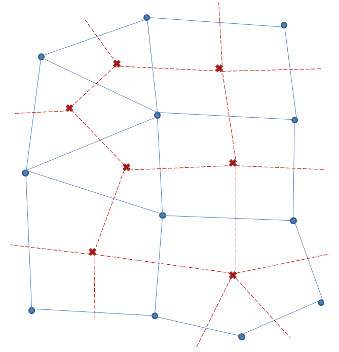
In the figure above, the grid nodes and edges are represented by dots and solid lines; the dual grid nodes and edges are represented by crosses and dashed lines.
From the mathematical point of view, sometimes the grid is augmented with a cell “at infinity” and analogously, the dual grid is augmented with a node “at infinity”. With these extra additions, the grid and its dual have some interesting properties. For instance, the dual edges intersect the regular edges and the two groups are in a one-to-one correspondence. Similarly, the dual cells are in a one-to-one correspondence with the grid nodes, and the dual nodes are in a one-to-one correspondence with the grid cells. Moreover, the dual of the dual grid is the original grid.
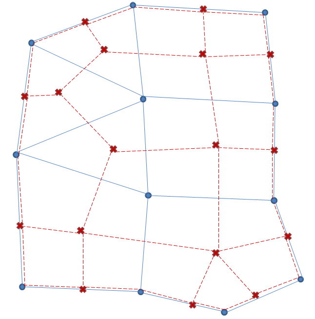
However, in the context of a numerical simulation, extending the grid to infinity is impractical. Therefore, the dual grid is truncated by adding dual nodes on the center of the boundary edges and dual edges along the boundary joining the boundary dual nodes. The one-to-one correspondences of the infinite model do not carry over to the truncated model, but some slightly more complex relations can be obtained. For instance, the dual nodes are now in one-to-one correspondence with the set of grid cells and grid boundary edges. For this reason, the boundary edges are considered as a sort of topological artificial cells with no area which are extremely useful when setting up boundary conditions.
In the context of the equations described in this document, it is convenient to numerically compute: the water surface elevation H at the grid cell centers (including artificial cells), the velocity perpendicular to the faces (determining the flow transfer across the faces), and the velocity vector V at the face points.