Hydrologic Unsteady Routing – Modified Puls - Example 19

This example will demonstrate the use of hydrologic unsteady routing in a HEC-RAS unsteady flow model. Modified Puls is the routing technique used to convey and attenuate the hydrograph downstream. This option is very useful when encountering portions of the model that are very steep and full unsteady flow routing is either unstable or not possible at all. A hydrologic routing reach can be an upstream piece, downstream piece, or an intermediate piece of any existing HEC-RAS unsteady flow river reach. It can also encompass an entire HEC-RAS river reach. When ran, the analyzer calculates and displays the hydrologic routing and unsteady flow portion of the reach simultaneously and seamlessly in one file. The modeler is referred to Chapter 6 of the User's Manual for a more detailed discussion on hydrologic unsteady routing.

To review the data files for this example, from the main HEC-RAS window, select File and then Open Project. Go to the directory in which you have installed the HEC-RAS example data sets. From the "Applications Guide\Example 19 – Hydrologic Routing - ModPuls" subdirectory, select the project labeled "ModPulsRouting." This will open the project and activate the following files:

Plan: "Modified Puls Upstream Run"
Geometry:"Existing Conditions – Modified Puls Upst"
Flow: "Flow Hydrograph No Dam"

Example 19 - Hydrologic Routing - ModPuls.zip

Geometric Data

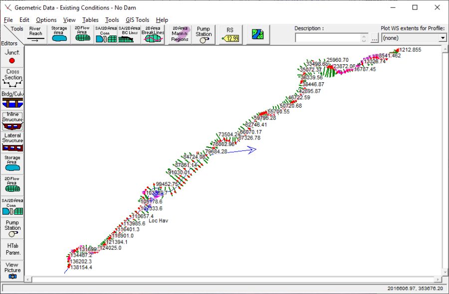
To view the geometric data for the river system, from the main program window select Edit and then Geometric Data. This will activate the Geometric Data Editor and display the river system schematic as shown in the figure below. The schematic displays the 177 river stations of the reach "Loc Hav" on "Bald Eagle" river, with river station 138154.4 as the upstream cross section and 659.942 as the downstream cross section. Information on entering and editing geometric data can be found in preceding examples as well as Chapter 6 of the User's Manual.

Unsteady Flow Data

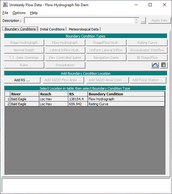
The user is required to enter boundary conditions and initial conditions for the system at the beginning of the simulation period. For additional information on unsteady flow data refer to Chapter 8 of the User's Manual, Performing an Unsteady Flow Analysis. The Unsteady Flow Data Editor, shown in the figure below, was selected from the main program window under the Edit menu.

Boundary Conditions

Boundary conditions are required for the farthest upstream and downstream cross sections. Upon entering the Unsteady Flow Data Editor the farthest upstream and downstream cross sections will be located in the boundary conditions column. In this case, the user will see River Station 138154.4 and River Station 659.942 as the upstream and downstream boundary conditions, respectively. Boundary conditions are set by highlighting the adjacent cell under Boundary Condition Type. When a cell is highlighted, not all boundary conditions are available. The program will automatically gray out all irrelevant boundary condition types. Internal boundary conditions may be added by selecting one of the buttons under the "Add Boundary Condition Location" heading.

Upstream Boundary Condition

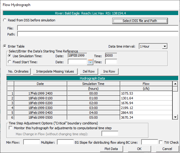
For River Station 138154.4 a flow hydrograph was selected by highlighting the cell and pressing the Flow Hydrograph button. The window where the Flow Hydrograph is entered is shown in the figure below. The user may select to read hydrograph data from a DSS file or manually enter the data. For further instruction on using a DSS file see Unsteady Flow Application Example 17. For this example the flow hydrograph was manually entered by selecting the Enter Table radio button. The Data Time Interval was set to one hour and the radio button Use Simulation Time was selected causing the initial propagation of the hydrograph to coincide with the beginning of the simulation time window. The hydrograph was then manually entered into the table.

Downstream Boundary Condition

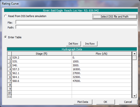
For River Station 659.942 the boundary condition selected was a rating curve. Again, the corresponding cell for that particular river station was highlighted and the Rating Curve button was selected. The window shown in the figure below is then displayed and the user is given a choice whether to Read from DSS before simulation or Enter Table. For this example the Enter Table radio button was selected and the stage and flow values were entered in the appropriate units.

Initial Conditions

Initial conditions consist of flow information at each of the specified cross sections, as well as elevations for any storage areas defined in the system. Data for initial conditions is established by selecting the Initial Conditions tab on the Unsteady Flow Data Editor. After selecting the tab, the figure below will be displayed.

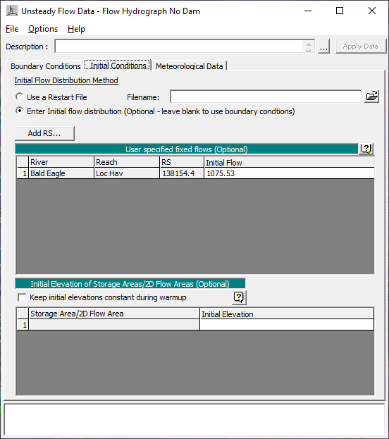
As seen in the figure above, the Enter Initial flow distribution radio button was selected and an initial flow of 1075.53 was entered for the most upstream river station (138154.4). The data was then saved (File -> Save Unsteady Flow Data As) in the Unsteady Flow Data Editor and the window was closed.

Steady Flow Analysis

Although the Modified Puls routing method is only used for unsteady flow, a steady flow dataset and analysis must be completed first. The purpose of the steady flow plan is to compute a range of water surface profiles that encompasses all expected flow rates of the unsteady model. The results from the steady flow run are used within the hydrologic routing reaches in order to provide the necessary discharge-volume relationships required by Modified Puls routing.

Steady Flow Data

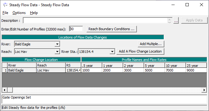
To enter the flow data, from the main program window Edit and then Steady Flow Data were selected. This activated the Steady Flow Data Editor as shown in the figure below. For this example, 30 flow profiles were computed ranging from a low flow of 1,000 cfs to a high flow of 60,000 cfs. A value of "30" was entered as the number of profiles and the central table of the editor established thirty columns for the flow profiles. The flow values were then entered at the upstream river station (138154.4) with values incrementally increasing by 2,000 cfs for each profile (with the exception of the last profile, which increases by 5,000 cfs).

The wide range of steady flow rates extends below the minimum (1,075.53 cfs) and beyond the maximum (50,000 cfs) flows within the unsteady flow hydrograph. If an unsteady flow rate is not encompassed within the range of the steady flow profiles, the model will calculate its corresponding stage by linearly extending the two nearest points on the rating curve and interpolating the stage value from the given unsteady flow value. Since the rating curve relationship of stage and flow is typically not linear, this interpolation is not recommended. Therefore, it is advised that the user uses a wide enough range of steady flow profiles so that all unsteady flows are included. Furthermore, a large number of water surface profiles (20 or more) are advised in order to get good definition in the rating curves.

Boundary Conditions

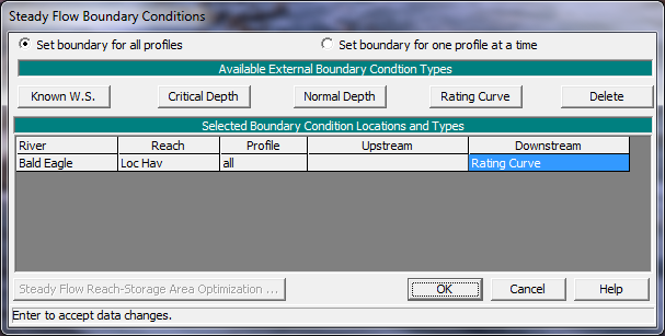
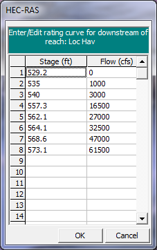
To enter the boundary conditions the Boundary Conditions button at the top of the Steady Flow Data Editor was selected. This activated the Boundary Conditions Editor as shown in the figure below (top). This flow analysis was performed in the subcritical flow regime. Therefore, a boundary condition was established at the downstream end of the reach for each flow profile. For a detailed discussion on the boundary conditions, the modeler is referred to Chapter 7 of the User's Manual and Chapter 3 of the Hydraulic Reference Manual. From the Boundary Conditions Data Editor, the boundary conditions were entered by first selecting the Downstream field and then Rating Curve. This activated a table where stage and flow information were entered as shown in the figure below (bottom). Once the data were entered, the OK button was selected to exit this window. This completed the necessary steady flow data for the analysis and the data were saved as "Steady Flow Data."

Steady Flow Computations

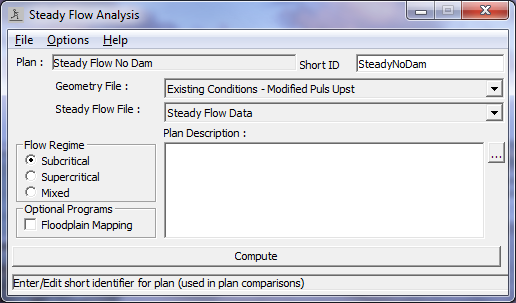
To perform the steady flow analysis, from the main program window Run and then Steady Flow Analysis were selected. This activated the Steady Flow Analysis Window as shown in the figure below. A Short ID was entered as "SteadyNoDam" and a subcritical flow analysis was selected in the lower left corner of the editor. The geometry file "Existing Conditions – Modified Puls Upst" and the steady flow file "Steady Flow Data" were saved as the plan "Steady Flow No Dam". A steady flow plan must be run using the exact same geometry file to be used for the unsteady flow modeling.

After all the necessary data was entered, the Compute button was selected to perform the steady flow analysis.

Hydrologic Unsteady Routing

The Modified Puls Hydrologic Routing editor is opened by selecting Options and then Hydrologic Unsteady Routing from the Geometric Data Editor. Once the Modified Puls window is displayed (below), the Use Modified Puls Routing box was checked on. If the Use Modified Puls Routing box is not checked, the Modified Puls routing option will be ignored, and HEC-RAS will perform full unsteady flow routing at all of the cross sections. However, when checked, Modified Puls routing will be performed on the specified cross sections when an unsteady flow analysis is run (it is ignored for steady flow runs).

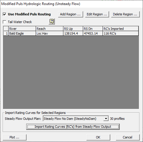
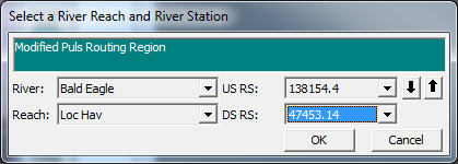
The cross sections for which Modified Puls routing was to be performed were selected by clicking the button Add Region and then choosing the upstream and downstream bounds of the river and reach which the routing was to be carried out (see figure below). Once the desired region was selected, OK was clicked. The region selected was automatically populated in the Modified Puls Hydrologic Routing table as seen in the figure above.

In order to populate the last column (RC's Imported), rating curves needed to be imported for the selected region. Below the table there is an area titled Import Rating Curves for Selected Regions where a list of steady flow output plans can be selected from a drop down menu. For this example, "SteadyNoDam" was selected and the number of profiles within the plan (30) was listed next to the drop down menu (see the first figure on this page). Next, the blank cell under the column heading RC's Import was selected. Then, Import Rating Curves (RC's) from Steady Flow Output was clicked and rating curves from the steady flow output were imported for all 116 cross sections within the designated region. The imported rating curves can be visually inspected by clicking Plot in the lower left hand corner of the window. It should be noted that the steady flow models should have been run previous to this step and that the same geometry file must be used.

Before clicking OK and exiting the window, the box corresponding to Tail Water Check was checked on. When turned on, this option will monitor the downstream interface of any hydrologic routing reach to verify that the next cross section downstream has a lower computed water surface elevation than the last section of the hydrologic routing reach. If it does have a lower computed water surface elevation then the results are accepted and displayed. However, if the downstream water surface (tailwater) is higher than the water surface of the last cross of the hydrologic routing reach, then the tailwater is forced into the downstream portion of the hydrologic routing reach. When run, the model will continue to overwrite the hydrologic routing cross sections' computed water surface elevations until a cross section is reached where the hydrologic routing computed water surface elevation is higher than the tailwater elevation.

Below are the water surface profiles from a similar geometry file as used in this example where the Tail Water Check was not used (top figure below) and where it was (bottom figure below). There is an inline structure in the middle of the reach that is causing a backwater effect upstream of the structure. As seen in the figure below, this backwater effect is only illustrated in the portion of the reach that is modeled as unsteady flow, while the portion modeled with Modified Puls does not consider the backwater effects of the inline structure, which causes the huge stage difference seen in the top figure below. By turning on the Tail Water Check, this unrealistic water surface profile is corrected by propagating the backwater effect upstream into the reach region that was modeled with Modified Puls routing.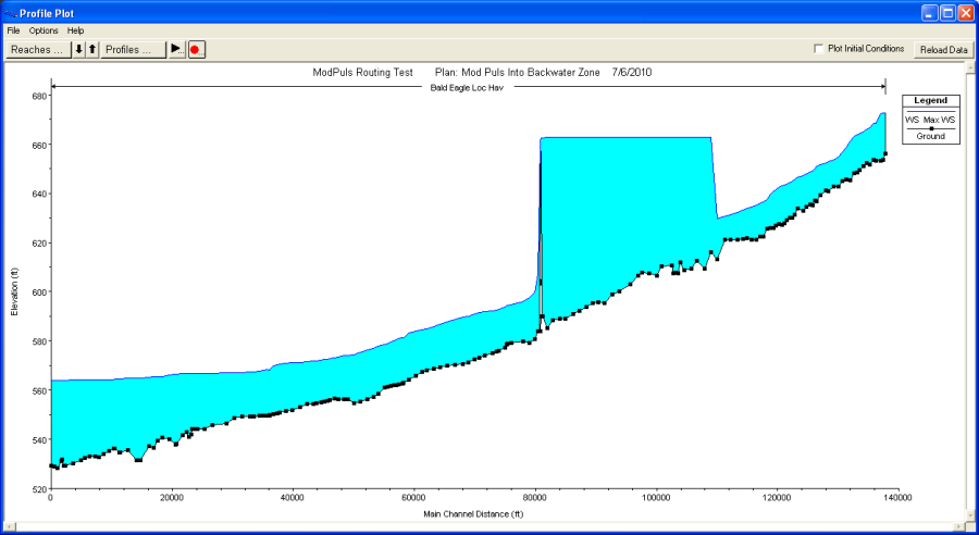

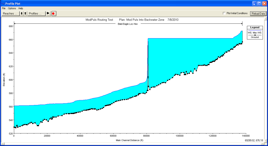
The Tail Water Check allows for downstream conditions to influence the water surface, volume, and flow rate in the hydrologic routing reach. Although the Tail Water Check function may give a more realistic result, it may also increase instability. It should also be noted that there must be at least one or two normal cross sections between the end of the reach and the Modified Puls region; if there isn't then the tailwater check will be ignored. For this specific example, the Tailwater check option was not used, because there were no downstream structures that will cause a backwater upstream in this example.

Unsteady Flow Analysis

After completing the preceding steps an unsteady flow analysis may be initiated. Under the main program window Unsteady Flow Analysis was selected under the Run menu. This will display the Unsteady Flow Analysis Window shown in the figure below. A plan was defined by selecting the Geometry File "Existing Conditions – Modified Puls Upst" and the Unsteady Flow File "Unsteady Flow." Under the File menu, Save Plan As was selected and the plan title was entered as "Flow Hydrograph No Dam." After entering the title of the plan a short identifier was entered as "ModPulsUpStream" and the plan was saved.

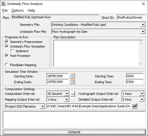
Simulation Time Window

The simulation time window, located on the figure above, requires a beginning and ending date and time for simulation. The date must have a four digit year and can be entered in the following format: 18FEB1999. The time field is entered in military time (i.e. 1 p.m. is entered as 1300). For this application the simulation time began and ended at 0000.

Computation Settings

The computation settings in the Unsteady Flow Analysis Window contain the following: the computational interval; hydrograph output interval; instantaneous profiles interval; and the name and path of the output DSS file.

For this example the computation interval was set to 30 seconds. In order to ensure stability and accuracy, the Courant condition was used to determine the computation interval (see Chapter 8 of User's Manual for more detail). The hydrograph output interval was set to 1 hour. This interval defines the output of computed stage and flow hydrographs written to HEC-DSS. The detailed output interval was set to 2 hours, specifying the interval at which detailed hydraulic output will be computed by the post processor. It is suggested that this interval remain fairly large to reduce the amount of post processing and storage required.

Programs to Run

There are three components used in performing an unsteady flow analysis within HEC-RAS: the geometric data preprocessor (HTAB); the unsteady flow simulator (UNET); and an output post processor. These three (plus Floodplain Mapping, which is not discussed in this application) can be found and turned on under the Programs to Run heading found on the Unsteady Flow Analysis window (see the figure above.

The geometry pre-processor is used to speed up the unsteady flow calculations by processing the geometric data into a series of hydraulic property tables and rating curves. It is highly recommended that the user run the geometry pre-processor and examine hydraulic output for anomalies before running the unsteady flow simulator and the post-processor.  The unsteady flow simulation is what actually creates the stage and flow hydrographs. The program is a three step process that requires the tables from the geometry pre-processer, the boundary conditions, and flow data from the interface to operate.

The post processor is used to compute detailed hydraulic information for a set of user specified time lines during the unsteady flow simulation period. By running the post processor, the user will have all of the available plots and tables for unsteady flow that HEC-RAS normally produces for steady flow. 

The Geometry Preprocessor, Unsteady Flow Simulation, and Post Processor were all checked on.

Location of Stage and Flow Hydrographs

The user has the option of specifying locations for which hydrographs will be computed and available for display. For this example the stage and outflow hydrographs were calculated for every cross section by clicking on Options then Stage and Flow Output Locations from the Unsteady Flow Analysis toolbar. A window opened and all 177 cross sections were selected by highlighting (All RS) and clicking the arrow to bring them over to the Selected Locations portion of the window. After selecting the cross section locations, OK was pressed.

Output Analysis

For the analysis of the output, the water surface profiles and the flow hydrographs will be reviewed. In addition, a comparison will be shown between this model run with full unsteady flow versus a combination of unsteady flow and hydrologic unsteady routing (as was used in this application). Each of these is discussed in the following sections.

Water Surface Profiles

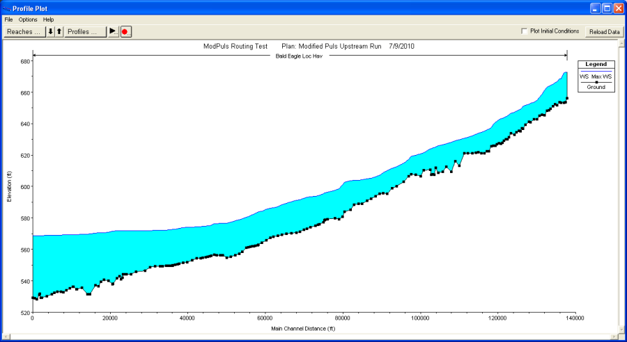
The water surface profiles are shown in the figure below. This figure was activated from the main program window by selecting View and then Water Surface Profiles. The figure shows the maximum water surface elevation. The entire event can be seen as an animation by selecting Options and then Animate from the profile plot window. As seen in the figure below, there is a smooth transition between the reach's upstream portion that was modeled with Modified Puls and the downstream portion that was modeled with the unsteady flow equations. If there were not a smooth transition the model would need to be reexamined to determine the cause. A good place to start is by evaluating the stage and flow hydrographs.

Transition from Modified Puls routing (upstream) to full unsteady flow (downstream).

Stage and Flow Hydrographs

The Stage and Flow Hydrographs can be viewed from the main program window by selecting View and then Stage and Flow Hydrographs. There are three different ways to view the stage and flow data: Stage Flow, Table, and Rating Curve. These viewing options can be selected from three separate tabs found above the output viewing window. Interpreting the stage and flow hydrographs is further discussed further in Chapter 9 of the User's Manual.

Full Unsteady Flow and Hydrologic Unsteady Routing Comparison

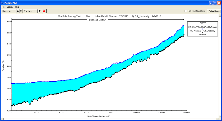
The Bald Eagle River modeled in this example application could actually be modeled entirely with the unsteady flow equations without going unstable. However, a portion of the river was modeled using the Modified Puls routing method so that the user could better understand how to utilize the feature. In order to convey the precision of the two methods (Modified Puls routing and the unsteady flow equations), they are compared here.

The discrepancy in water surface elevations between the two methods is negligible for this example – most cross-sections show a difference within a couple of inches or less. The figure below shows the close proximity of the maximum water surface profiles of the Modified Puls run (straight blue line) and the full unsteady run (blue line with triangles). Yet, there are some instances such as during low flows or when channel contraction occurs near a bridge when there are larger discrepancies. These differences are primarily because the hydrologic modeling method doesn't completely capture the hydrodynamics associated with the changes in flow rate like the unsteady flow equations do.

Summary

The Hydrologic Unsteady Routing option is very useful when encountering portions of the model that are very steep and full unsteady flow routing is either unstable or not possible at all. To perform the analysis the user must enter the geometric data for the river reach. Within the Geometric Data Editor the hydrologic unsteady routing parameters are entered. A steady flow model must be created using the exact same geometry file to be used for the unsteady flow modeling and should include a set of profiles that includes all possible flows within the unsteady flow model. The rating curves from the steady flow output are imported into the Modified Puls Hydrologic Routing Editor so that stages and flows can be interpolated when it is evaluated in the Unsteady Flow Analysis. Although unsteady modeling is more accurate than Modified Puls routing, there is typically very little variance between the results.