The Rouse-Diffusion method uses three analytical equations to compute 1D floodplain deposition.

1. First, it uses the Rouse equation to compute how much of each grain class is available for floodplain deposition. 
2. Then it uses a diffusion equation to compute how much of that available sediment can diffuse out to each floodplain node. 
3. Finally, it does a mass balance and fall velocity analysis to determine how much of the floodplain concentration can deposit at each node.  

This method offers three main advantages over the veneer method.  

1. First, it limits floodplain deposition to suspended load.  Grain classes that are entirely (or mostly) bed load will not deposit in the floodplain.
2. Second, it computes non-uniform lateral floodplain deposits.  The algorithm deposits more sediment closer to the channel, forming natural levess and thinner deposits farther from the bank.
3. Third, it decouples floodplain deposition and channel deposition.  By removing floodplain sediment from the Exner equation and then applying the Exner equation only to bed-material load in the channel, it avoids some of the numerical artifacts that arise from applying the Exner equation to the channel and floodplain simultaneously.

However, this method also has one major liability:

This Method Does Not Account For Floodplain Advection

This method does not account for floodplain deposition by advection.  Because this algorithm is in the 1D model, the model has no mechanism to consider 1D advection.  But advection is often an order of magnitude more important for floodplain deposition (Pizzuto, personal communication).  Therefore, using a diffusion model to simulate 1D floodplain deposition under-predicts the process and becomes a heuristic for a larger suite of processes.  This will be a better approximation in some systems than others.  If the diffusion assumption breaks down in your model, consider moving to a 2D sediment transport model.

Step 1: Computing Floodplain Available Concentrations

First, HEC-RAS uses the Rouse (1937) distribution to compute a vertical concentration distribution for each grain class.  

This analytical distribution compares the shear velocity (u*) to the fall velocity (w) in a dimensionless parameter called the Rouse Number:

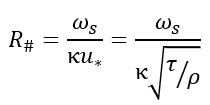
where K is the dimensionless von Karmen coefficient (~ 0.4) and u* is the square root of the ratio between shear stress and fluid density.

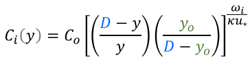
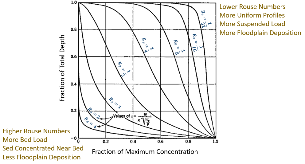
The smaller the rouse number is, the more uniform the vertical concentration profile is (i.e. concentrations near the surface are closer to concentrations near the bed).  The larger the Rouse Number is the more transport is concentrated near the bed.  Rule of thumb approaches sometimes suggest that Rouse Numbers > 2.5 mean that the grain class is primarily bedload, Rouse Numbers <0.8 indicate wash load, and the zone between those include some combination of bed and suspended load.  But the actual distributions are more continuous.    In the analytical distribution, the rouse number becomes the power of a relationship between the computed depth (y), the total depth (D), and the "reference depth" (yo)- a distance above the bed where a reference concentration (Co) is measured or known.

This generates the classic, unit, concentration profiles in the following diagram (each labeled with the associated Rouse number), plotted as a vertical fraction of the total depth and a horizontal fraction of the maximum concentration.

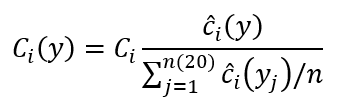
HEC-RAS already computes a concentration for each grain class in each control volume with the transport functions, so it does not use the reference concentration approach.  It uses the Rouse distribution to distribute those computed concentrations and determine the fraction of sediment that is transporting above the bank stations.  Therefore, it computes a unit Rouse profile with the approach illustrated in the figure below.

Then the algorithm scales the unit Rouse distribution so the mass represented in the Rouse profile equals the mass computed by the transport function (Ci). 

Then the model integrates the concentration in the portion of the water column between the bank elevation and the water surface elevation (for each grain class).  That concentration is the "floodplain available" concertation (Cfp).  Floodplain deposition for each grain class is limited to the sediment between the bank elevation and the water surface elevation.  Therefore, the Rouse component of this algorithm will mostly exclude coarse material (with high fall velocities and large Rouse numbers that transport as bedload) from floodplain deposition. 

ASCE Retrospective on The Career of Dr. Hunter Rouse

Dr. Hunter Rouse, the source of the Rouse distribution is one of the important figures in sediment transport.  ASCE did a retrospective on his career that is worth reading:  

Ettema, R. "Hunter Rouse - His Work in Retrospect," ASCE Journal of Hydraulic Engineering, 132(12), https://doi.org/10.1061/(ASCE)0733-9429(2006)132:12(1248) 

Step 2: Distribute Floodplain Available Sediment Across Floodplain

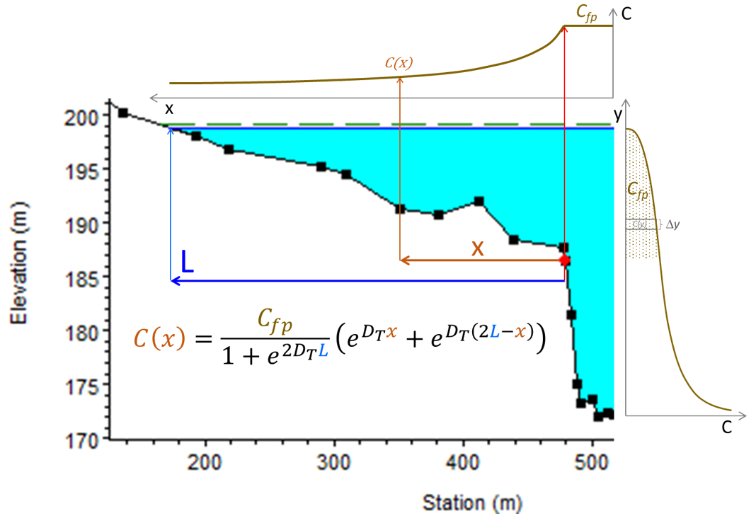
After HEC-RAS computes the floodplain-available concentration for each grain class, the algorithm uses an analytical diffusion equation to distribute that concentration laterally, across the wet nodes of the floodplain.  HEC-RAS uses an equation developed by Yotsukura and Cobb (1972) and applied to sediment in Pizzuto (1987): 

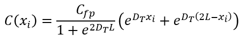
where the variables and parameters are defined in the following figure.  C(xi) is the concentration at each station-elevation point (i), L is the wet "length" (lateral width) of the floodplain, x is the horizontal distance between each floodplain station-elevation point (i) and the channel bank, Cfp is the floodplain available concentration computed from the Rouse algorithm (Step 1) and DT is the diffusion coefficient.  This analytical distribution computes a concentration "decay" process, as less sediment transports farther from the channel.  DT is the diffusion parameter exposed to the user.  Increasing DT makes more sediment available at the farther floodplain nodes.

Select Bank Stations and Movable Bed Limits Carefully

The Rouse component of this algorithm is sensitive to the elevation of the hydraulic bank station (not the movable bed limit) and the diffusion component is sensitive to the station of the bank station.  It is always important to select bank stations carefully in 1D sediment models.  But selecting bank stations that reflect the actual transition from channel flow-to-floodplain flow is especially important in this method.  Additionally, if you use the Rouse-Diffusion floodplain method, set the movable bed limits at or inside of the bank stations.  The algorithm will use the floodplain method outside the bank stations and the Exner equation inside the movable bed limits.  If the movable bed limits are outside the bank stations, those nodes will be subject to both processes which will double-count and may lead to strange numerical artifacts and cross section shapes.  

Step 3: Compute Deposition at Each Station-Elevation Point

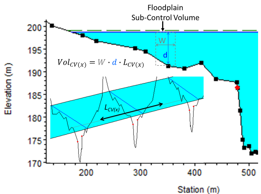
Next, HEC-RAS must convert the concentration at each station-elevation point into a depositional mass, to determine how much to raise the node elevation.  The algorithm builds a control volume around each wet, floodplain, station-elevation point (see following figure). 

It is good modeling practice to select a time step that achieves a “Sediment Courant Condition” close to 1; the sediment travels through a control volume in one time step.  However, because different grain classes have different transport velocities at different flows, most models do not have universal, sediment, Courant number.  During each sediment time step, the water volume that passes through a control volume can be much greater or much smaller than the control volume itself.  To estimate the mass of sediment that has an opportunity to deposit at each cross-section node in a time step, the model must compute the water flux that passed over it.

First HEC-RAS computes the scaled water flux through the local control volume, which is the water flux through the whole cross section, scaled by the static volume ratio of the local control volume to the water volume in the whole-XS control volume.

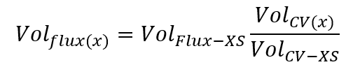
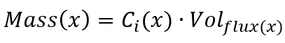
Then HEC-RAS computes a sediment flux passing over the station-elevation point in a time step by combining the local water flux and the concentration at that location from Step 2:

Once HEC-RAS computes the mass available at each floodplain station-elevation point in a time step, it is a simple matter of comparing the residence time to the fall velocity of each grain class to compute deposition.

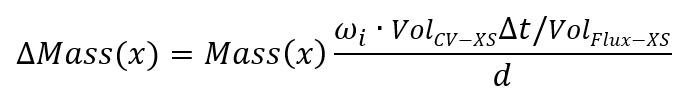
Then, the mass change (deposition) can be divided by the local, control-volume area (W*LCV in the previous figure) to compute elevation change for the floodplain node.

___________________

For more information on how to use this method, see the appropriate section of the User Manual  

References

Pizzuto, J.E. (1987) “Sediment diffusion during overbank flows.” Sedimentology, 34, 301-317.

Rouse, H. (1937) “Modern conceptions of the mechanics of fluid turbulence.” Transactions of the American Society of Civil Engineers, 102, 463–541.

Yotsukura, N. and Cobb, E.D. (1972) "Transverse diffusion of solutes in natural streams." USGS Professional Paper 582, 18p, DOI: 10.3133/pp582C.

This Draft RSM Tech Note (Gibson et al., 2022 - In Review) also describes these methods.