Modeling Note: Developing Long-Term Temperature Records
Temperature data are seldom sufficient to generate a daily time series for multi-decadal, historical models. And modelers must make some temperature assumption to simulate the future. There are a few options to define multi-decadal historical or future temperature data in the absence of a long-term temperature record (Options 1 and 3 are most common):
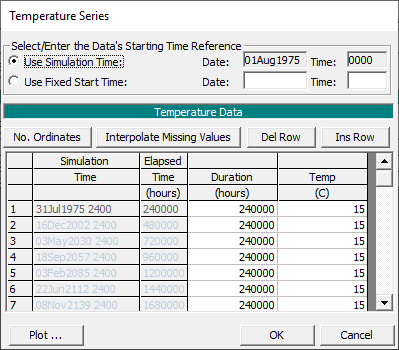
- Constant Temperature: Any of the irregular time step editors in the quasi-unsteady flow boundary conditions can define a constant condition by specifying large durations (e.g. 240,000 hrs or 10,000 days/>25 years in the figure below). In coarse systems (rivers with significant gravel and/or cobble), that are less sensitive to temperature, detailed temperature data may be unnecessary. Perform sensitivity analysis to evaluate this assumption.

- Interpolating Annual Highs and Lows: If results are sensitive to temperature, HEC-RAS can generate a simple time series with a little more user effort. Estimate max and min water temperatures and input them at approximate dates each year, leaving the intermediate dates blank. Then press the Interpolate Missing Values button (below). For example a user could create a weekly time series (Durations=7*24 hrs = 168 hrs) that interpolates between an early July high and early December low by defining the high temperature in all of the rows aligned with the first week of July, the low temperature with all the rows associated with the first week of December, and pressing the Interpolate Missing Values button.

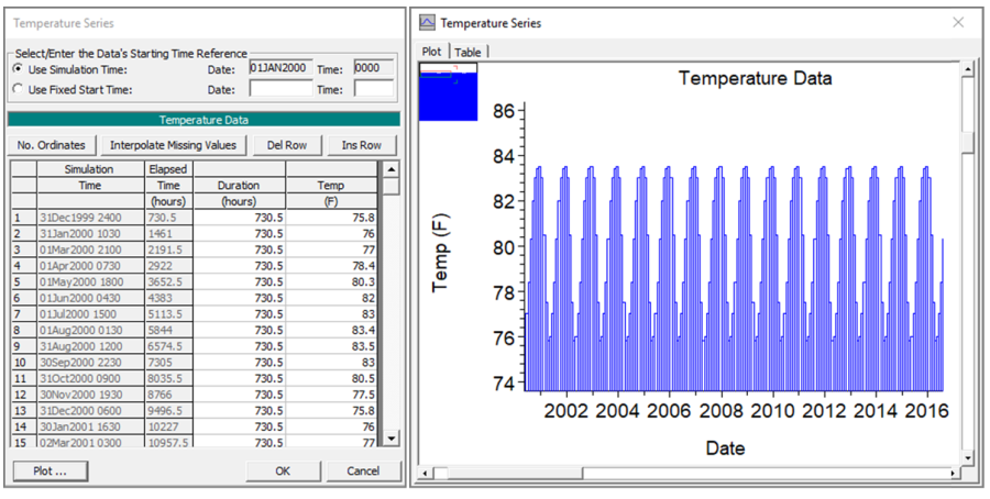
- Monthly Average Temperatures: Often a gage has some opportunistic temperature readings. You cannot use them as a times series or even interpolate a time series from them. The gage has enough water temperature data to compute monthly averages. Give each monthly average temperature a 730.48 hour (30.4368 day) durations will create an approximate average monthly temperature time series that you can repeat for multiple years (demonstrated in figure below) and it will remain relatively consistent over long simulations (including leap years).
