Averaging Low Transport Time Steps

The computational increment can subdivide Flow Durations (e.g. daily average flows) into smaller time steps to evaluate bed change feedbacks on hydraulics more frequently. However, modelers sometimes want to "go the other way" with their time steps, and combine multiple flow durations into a single computation increment (e.g. combine seven daily, low-transport, summer flows into a weekly time step).

Combining low-flow/low-transport time steps to reduce run times is a relatively standard practice (though it was more standard 10-20 years ago when computational power was more limiting). But modelers should consider the implications of transport non-linearity when averaging flows for a sediment transport model.

Consider two unit less flows (100 and 200) a simple sediment rating curve, where:

Averaging the flows, and then using the average flow to compute transport will yield a different result than computing the loads and then averaging the loads. However, the latter is likely more correct.

Average Flows First

Compute Loads First

These errors might be small (though, over a 50 year simulation, they can add up, particularly if the averaging is aggressive), but it is more important to conserve sediment mass in a quasi-unsteady sediment model than water volume. Therefore, when averaging flows for a sediment model, the best practice includes computing loads for those flows, averaging the loads, and then backing out a flow that produces the average load.

This process also can be more important when the flow data is sub-daily. For example, one year of 15-minute data will nearly fill the available rows (4*24*365=35,040) in the quasi-unsteady editor and make run times unacceptable. It used to be impossible to run multiple years of 15-minute flow data in quasi-unsteady flow because the data simply would not fit in the editor. Now users can attach and run as many years of 15 minute data as they have by specifying it as a DSS boundary condition. However, run times will still make this impractical for most models. Therefore, it is critical to combine low (and moderate) flows for high resolution flow time series.

If this sounds like a lot of work, the Histograph Generator may be able to help.

The Histograph Generator Tool

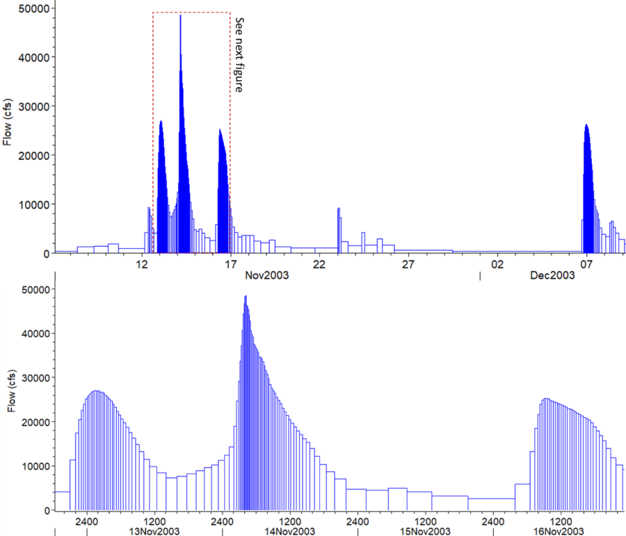
Because sediment transport is non-linear, and high transport periods can punctuate long periods of low transport that may be morphologically insignificant, sediment modelers often want to optimize their time step. Particularly when computers were slower, modelers wanted to group low flow time periods into long computation increments to save run time. This practice is less common now that computers are faster, but period of record simulations can still have significant run times. Therefore, the histograph generator provides a tool to determine the time step based on the sediment flux. It scales the flow durations to bring in an equal, user specified, load over each flow period, which could be a few seconds at the peak of the flood of record, or a few weeks during a drought (below). These irregular, equivalent load, flow durations can then be sub-divided by the computational increment for model stability.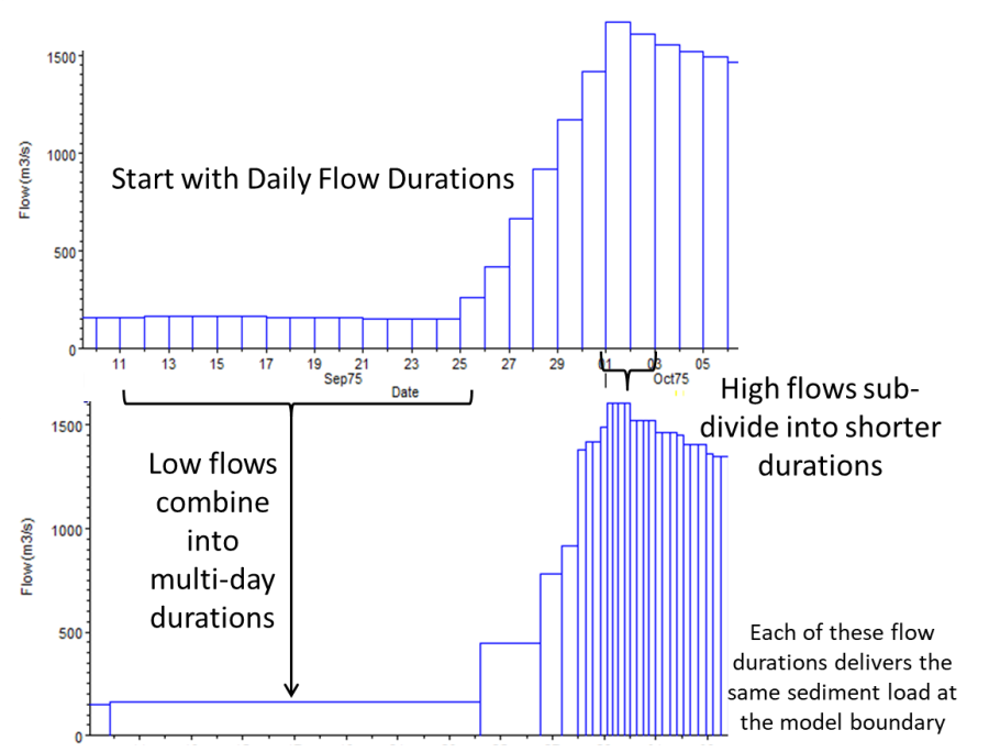

The Histograph Generator creates a new quasi-unsteady flow file with an irregular flow duration. If the histograph tool combines flows, it computes the flow that generates the average sediment flux (instead of the average flow). To launch the tool, select the Histograph Generator button on the Quasi-Unsteady Editor, from the base quasi-unsteady flow file. To launch this tool, press the Histograph Generator button on the Quasi-Unsteady flow editor (below).

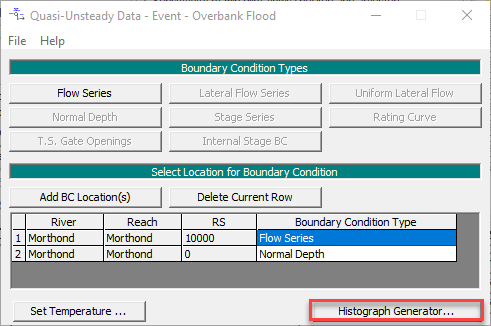
HEC-RAS requires two user inputs to create an equal-load increment flow file: a constant load and a flow-load rating curve.

First, the tool requires a user-specified load (below). Define the load that will determine the duration of each time step. The Histograph generator will use the flow-load relationship to determine how long each time step will be.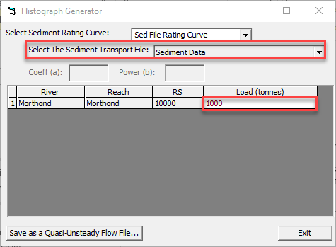

Second, the tool requires a relationship between flow and load. There are three options to define a sediment rating curve:

Sediment File Rating Curve:

If you have created a sediment transport file with a rating curve boundary condition, the Histograph generator can use that file directly. Select Sed File Rating Curve and then use the dropdown box labeled Select The Sediment Transport File (figure under Power Function:) to pick the sediment file with the appropriate rating curve boundary condition.

Power Function:

If the sediment relationship can be defined by a single power function, HEC-RAS can compute load data for the flow series from a simple power function, defined by two coefficients, where:

Select "Power Function" and define the two coefficients in the fields depicted in the figure below:

User Defined Rating Curve:

Finally, users can enter a flow-load rating curve directly into the histograph tool by selecting Define Rating Curve (below). This can be particularly useful for "bent" or "inflected" rating curves that cannot be described by a single power function.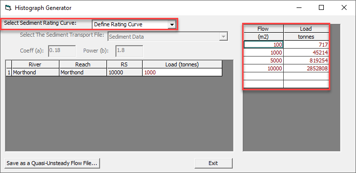

Creating a New Equal-Load Time Step Quasi-Unsteady Flow File

Once the load increment and the flow-load relationship are specified, press Save as a Quasi—Unsteady Flow File. This will launch a Save-As dialogue prompting the user to give the new quasi-unsteady file a name. Name the file and press OK.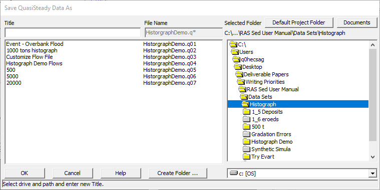

This simply adds the computed histograph to the project as a new quasi-unsteady file. Open the quasi-unsteady file in the quasi-unsteady editor. This file will only have an upstream flow boundary condition. Open that flow boundary condition and press Plot to review the histograph.

Preserving Low Flow Computational Increments

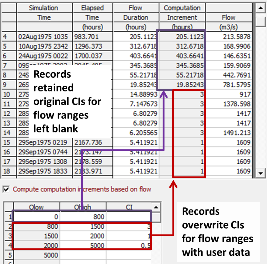
The tool only computes equal-load Flow Durations so it sets the Computational Increments equal to the durations. Users can edit the computational increments to sub-divide the high flows further. However, this is tedious to do manually. The option to Compute Computational Increments Based on Flow can be a helpful tool to automate that.

But if users want to subdivide high flow durations but keep the computational increments equal to the flow duration for lower flows, they need to use this tool in a particular way. The tool was designed to NOT overwrite computational increments in flow ranges left blank for this particular purpose. So in the example in the figure below, flow records between 0 and 800 cms keep the Computational Increment from the histograph analysis (= the Flow Duration, so HEC-RAS runs it in one sediment time step) and those >800 cms get the user specified sub-divisions.  Includes an example of a 15-minute flow series converted into an equal-load increment qausi-unsteady flow file (from Gibson and Helminiack, 2020).

Modeling Note

This tool is available but not widely used for daily data. For most studies, the computational expense of running daily flows during low-transport months is acceptable. But it becomes very useful if the flow data comes in 15-minute increments.

Modeling Note: Testing the Histograph

It is important to test the histograph against the base flow file to make sure it reproduces the results.

Modeling Note: Multiple Upstream Boundary Conditions

The histograph generator works best for models with just one upstream, sediment boundary condition. Dendritic models will populate multiple load fields to specify and the tool will try to find a common denominator, but stripping the analysis to a single boundary flow and load relationship will usually yield better results.

Modeling Note: 15 Minute Tidal Data

The other data that sometimes come in 15-minute increments are tide data. Again, the 40,000 maximum rows in the stage editor will not hold much more than 1 year of 15-minute data. So tidal stages must be averaged. Depending on the model objectives, some simulations can use a single representative stage, and other use a 6-hour representative stages (not necessarily averages) around the maximum and minimum cycle. However, downstream stages have non-linear effects as well, that are more difficult to tease out. It is a good practice to run a year of the sediment transport simulation with the 15-minute stage data and the proposed simplification to make sure the simplification reproduces the full time series.

Wish List

Wish List – Currently, the historgraph generator is built around the "equal mass per time step" principle. However, it would be useful to have simpler, more flexible, averaging tools available that create flow series based on load conservation principles, but are not constrained to the constant load approach. We would like to add a simpler feature that retains the flow duration and computational increments selected above a specified flow and simply combines low flows (under a certain threshold – or combines different flow ranges into different. We'd also like to add a DSS record to the downstream stage series editor and average it at the dynamic scale of the flow computational increment.

Wish List

Wish List – Plotting feature that plots the result before it writes to a new Quasi-Unsteady file. At this point users have to create a new quasi-file and open it to evaluate the load increment and results. A Plot feature would run the analysis and plot the result without creating the file, which would be quicker and cleaner.