Download page Automated Calibration of Manning’s n Values for Unsteady Flow.
Automated Calibration of Manning’s n Values for Unsteady Flow
In order to assist engineers in the calibration of unsteady flow models, we have added an automated Manning's n value calibration feature. This Option requires observed stage time series data (flow time series is optional) in order to be used. Manning's n values are calibrated on a reach basis. One or more reaches can be calibrated within the same run. Hydrographs are broken into flow zones from low to high in order to allow Manning's n values to vary with flow rate. The results from using this feature are a set of flow versus roughness factors for each reach that it is applied too.
This automated calibration feature can be applied in either a "Global" or "Sequential" optimization mode. The "Global" mode optimizes Manning's n values for all reaches at the same time. While the "Sequential" mode optimizes Manning's n values for one reach at a time, working from upstream to downstream. Manning's n values are optimized (adjusted) for each flow zone until the maximum flow zone error is less than a user entered tolerance, or until a maximum number of iterations is reached.
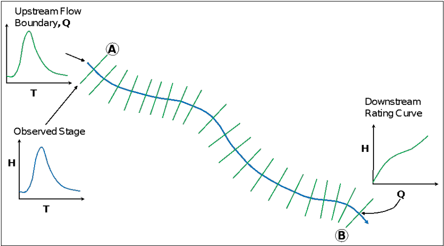
To better understand how this works; let's look at the optimization procedure for a single reach, as shown in Figure 14-85. Figure 1485. Single Reach Example
For the single reach example shown in Figure 14-85 above, there is a flow hydrograph introduced as the upstream boundary condition and a rating curve used as the downstream boundary for the reach. An observed stage hydrograph is attached to the model at the most upstream cross section (labeled as location A). Location A is where the software will compare the computed stages to the observed stages, in order to make decisions on how to change the Manning's n values for the reach. The user must set up a flow versus roughness factor table for the reach to be calibrated (optimized). For this example, let's assume we will have the entire reach set up as a single flow versus roughness factor reach. The user will enter flows versus roughness values into a table. The hydrograph is broken into flow zones from low to high in order to allow Manning's n values to vary with flow rate (Figure 14-86). The number of flow values entered in the flow versus roughness factor table will dictate how the hydrograph is broken up into flow zones for that reach. The roughness factors can be entered simply as values of 1.0 to start out, which assumes no change to the base Manning's n values. The optimization process will adjust the flow roughness factors for each flow zone in order to improve the model calibration.
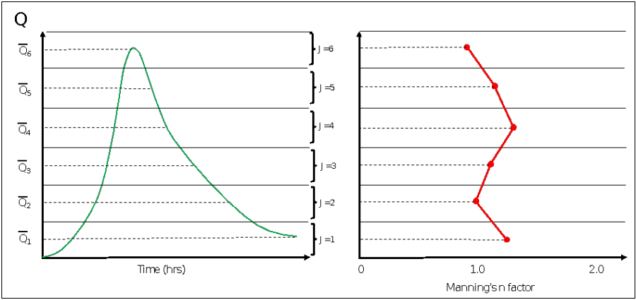
Figure 1486. Flow Zones Versus Manning's roughness factors.
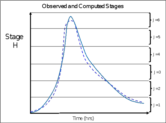
As shown in Figure 14-86, the hydrograph for this example is broken into 6 flow zones (this is controlled by the user). The software first runs the entire analysis just using the base Manning's n values (those entered by the user in the Geometric data editor). Then the computed versus observed stages are compared for each flow zone (Figure 14-87). The model adjusts roughness for each flow zone depending on the magnitude and direction of the error in that flow zone. The product of the optimization run is a set of Flow versus roughness factors that best fits the observed data given the information provided. Figure 1487. Computed and observed stages broken into flow zones for comparison.