Download page Viewing Computational Level Output for Unsteady Flow.
Viewing Computational Level Output for Unsteady Flow
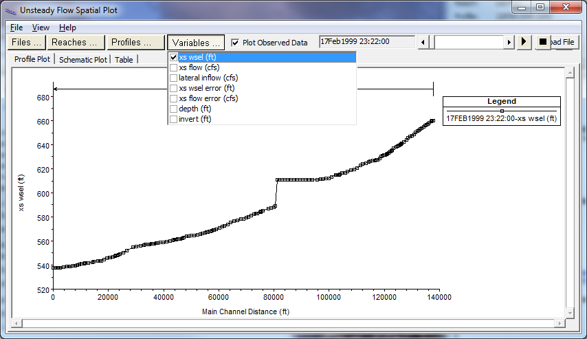
When performing an unsteady flow analysis the user can optionally turn on the ability to view output at the computation interval level. This is accomplished by checking the box labeled Computation Level Output on the Unsteady Flow Analysis window (In the Computations Settings area on the window). When this option is selected an additional binary file containing output at the computation interval is written out. After the simulation the user can view computation level output by selecting either Unsteady Flow Spatial Plot or Unsteady Flow Time Series Plot from the View menu of the main HEC-RAS window. Shown in Figure 8-28 is an example of the Spatial Plot. Figure 828. Unsteady Flow Spatial Plot for Computational Interval Output
As shown in Figure 8-28, the user can view either a profile plot, a spatial plot of the schematic, or tabular output. The user can select from a limited list of variables that are available at the computation level output. These are water surface elevation (XS WSEl); Flow (XS Flow); computed maximum error in the water surface elevation (XS WSEL ERROR); computed maximum error in the flow (XS FLOW ERROR); and maximum depth of water in the channel (DEPTH). Each of the plots can be animated in time by using the video player buttons at the top right of the window. This type of output can often be very useful in debugging problems within an unsteady flow run. Especially plotting the water surface error and animating it in time.
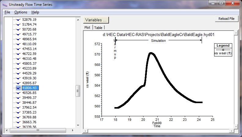
The other type of plot available at the computation interval output level is the Unsteady Flow Time Series Plot. When this option is selected the user will get a plot as shown in Figure 8-29. Figure 829. Unsteady Flow Time Series Plot at Computation Interval Level
As shown in Figure 8-29, the user has the option to plot or tabulate the time series output. Additionally, the user can select from five variables to display on the plot/table. The variables are chosen from the Variables button at the top of the window.