Download PDF
Download page Analytical and Tabular Rating Curve Results.
Analytical and Tabular Rating Curve Results
After the analyses and visualization, modelers and analysts eventually will want to reproduce the rating curve. To get the rating curve results, go to the Results tab (that is grouped with the Controls in the standard layout).
This tab provides two types of results:
- Regression Results that will help reconstruct an analytical power function and
- Rating Curve Output, which computes the loads for user specified flows in a tabular format
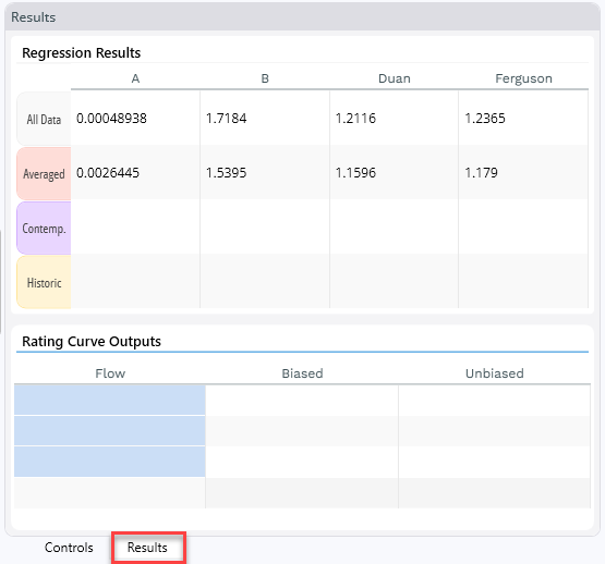
Regression Results (Analytical Results)
The Regression Results provide the ingredients to reconstruct the
By default, the tool computes the unbiased regression (with both correctors) for all the data and the temporally averaged data. The tool offers these regressions by default because averaging replicates and bias correction are best practices for most applications. The parameters fit the equation
Qs = E a Q b
where Qs is the sediment load (or concentration if the analysis used concentration), a and b are the coefficient and the power, and E is the bias corrector (Duan or Ferguson). So, the results in the figure above translate into an analytical rating curve of:
Qs = (1.1596) 0.0026445 Q 1.5395
with the Duan correction of the temporally averaged data.
Regression Results from Stationarity Analysis
If you use the Stationarity Control (e.g. the results below are associated with the stationarity control bar also pictured below) the analytical rating curve results will also populate the coefficients for the "historic" and "contemporary" regressions. The historic regression includes the data before the split-year selected in the stationarity scroll bar and the "Contemporary" coefficients reproduce the power function fit to the data points more recent than the stationarity threshold.
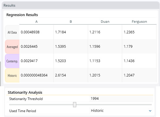
For example, in this analysis, the measurements before 1994 (with the Duan correction) yield a rating curve of:
Qs = (1.2015) 4.836E-8 Q 2.6154
while the data after 1994 (with Duan) yield:
Qs = (1.2015) 0.002941 Q 1.5203
Piecewise Linear Regression Does Not Have an Analytical Result
Because the piecewise linear regression is actually two power functions forced to connect within the data domain, it cannot be characterized by a single set of power-function coefficients. Use the below feature (the tabular rating curve) to generate a piecewise rating curve (and make sure you select one point at or very close to the inflection point).
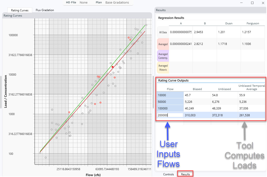
Generating a Tabular Rating Curve (Tabular Results)
HEC-RAS sediment, rating-curve boundary conditions require a tabular flow-load or flow-concentration rating curve. An example of a flow-load rating curve boundary condition in the HEC-RAS sediment model is included below.
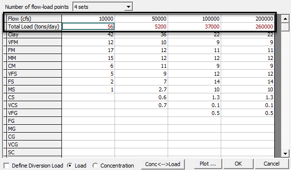
The tabular data requires user input. It is blank by default. The user must input flows (see figure below). When the user inputs flows, the tool will compute loads with the active methods (the methods used in the Control menu). In the example below, the user input four flows and the tool returned the biased and unbiased results, assuming all measurements were independent and the unbiased results (with the method selected in the Controls menu - Duan in this case) with temporal averaging. The tool returns the Unbiased, Temporally Averaged results by default, because these are considered best-practice for most systems. These results were transposed into the HEC-RAS sediment boundary condition above.
Logarithmically Interpolate Between Tabular Results
The tabular results reproduce the rating curve with two or more points. To compute loads for other flows, modelers and scientists will have to interpolate between these flow-load pairs. But these are logarithmically distributed data that fall along a power function (log transformed linear relationship). A simple linear interpolation is not appropriate. HEC-RAS log-interpolates between these data. Other applications should as well.
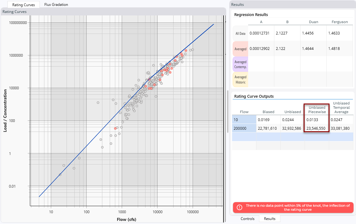
Piecewise Linear Result
Flow-load power functions can be defined with two points (these points should bound the highest and lowest flows expected, not the highest and lowest flows observed in the data). But a piecewise linear result requires at least three, and should include a point at or very close to the inflection point (i.e. the "knot"). For example, in the result below, the user has only entered bounding flows (high and low) in the tool. The tool is providing an error message, that to get good results from the piecewise linear tool, they must include a flow close to the inflection point (or knot).
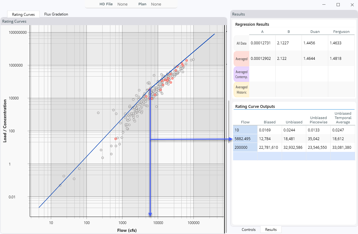
When the user copies the inflection point for the piecewise linear analysis into the flow data, the tool generates a three-point curve and the error goes away.
Wish List - Local Regression
We would like to add LOESS local regression analysis to fit independent but continuous non-linear relationships to different portions of the curve. These approaches do not devleop simple analytical equations, but could generate tabular results that could feed a model.