Sampling programs sometimes take multiple sediment measurements in a single sampling event. Because of sediment's natural variability, these sediment loads can vary dramatically, even though they were collected a few minutes or hours from each other and at about the same flow. The gage below includes a number of these multi-measurement, same-day replicates.
The vertical "striations" in the data often indicate these kinds of same-day replicates.
Regression analysis assumes each observation is independent. But these same-day replicates often are not. In this gage, the historical data mostly include single sample measurements. Therefore, if the regression analysis considered each contemporary replicate as an independent sample, it would overrepresent these data.
Temporal Averaging
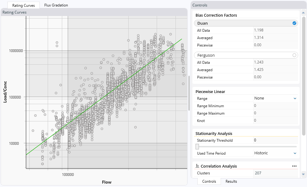
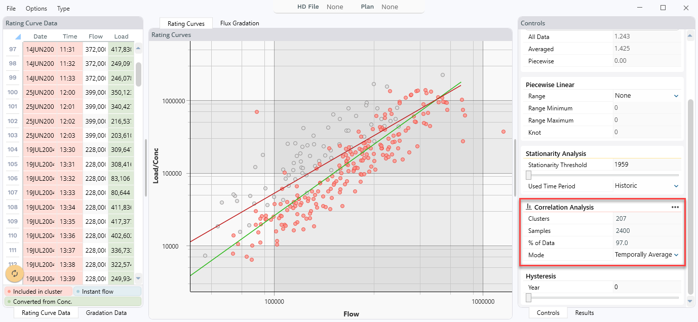
The temporal averaging/autocorrelation tool allows users to automatically average replicates collected within a specified time frame. This control reports the number of "clusters" which are the collections of replicates that fall within the specified time threshold of each other (12 hours by default). At this gage, 2400 measurements fall within 12 hours of another measurement, and they group into 207 12 hour clusters. 97% of these data were collected as multi-measurement replicates within a single sampling event.
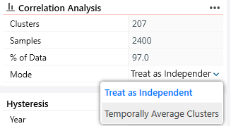
The Mode provides two options. The tool plots all the data and computes the regression as if they are independent by default. This can be appropriate for small rivers with flashy hydrographs, where samples collected in close succession have very different flows. But for large rivers, it is almost always appropriate to average these temporal clusters.
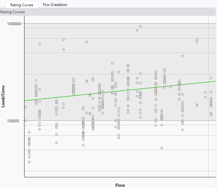
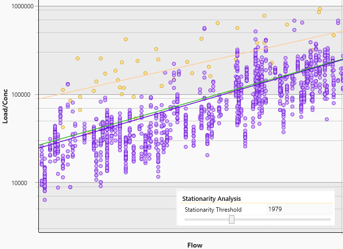
At this gage, averaging the clusters reduces the power of the contemporary measurements and generates a higher rating curve (though the analyst should also note the non-stationarity and decide if it is appropriate to use all of the data). The plot replaces the replicates with the cluster-average loads or concentrations (red). The Sediment Rating Curve Analysis tool also marks the measurements that fall within the time tolerance of other measuremnts in the data grid.
Setting the Temporal Averaging Threshold
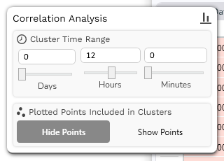
By default, the temporal averaging tool averages observations collected within 12 hours of each other. But that time threshold is variable.
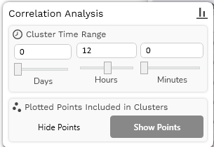
To change it, go to Options → Correlation Analysis.
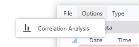
This opens an editor that allows users to set the temporal averaging threshold.
Plotting Original and Averaged Points
By default, the temporal averaging tool only plots the average measurements. However, under Options → Correlation Analysis users can select Show Points. This plots both the average and the averaged data so users can see the original measurements.
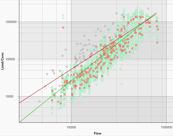
The plot below includes single-measurement observations (grey), replicates (green) and replicate cluster averages (red). The green line is the unbiased regression for all of the measurements. The red is the unbiased regression of the single-measurement observations and the temporal averages.