Download PDF
Download page Stable Channel Design.
Stable Channel Design
Stable channels can be computed using three different methods:
- Copeland
- Regime
- Tractive Force
To access the stable channel design window, click on Type…Stable Channel Design in the Hydraulic Design Window. The following window will become active:
Stable Channel Design Window
Copeland Method
Dr. Ron Copeland developed the "Copeland Method" (aka the Stable Channel Analytical Method) as a simplified tool to screen channel restoration alternatives. It is a useful method to quickly evaluate a range of possible slope-width-depth combinations that are likely to remain in relative continuity with the sediment transport (e.g. less likely to erode or deposit). The method combines a sediment transport function (Brownlie) with a roughness equation to compute a suite of slope-with and slope-depth pairs that would be in rough continuity with the computed sediment load.
To use the Copeland Method, select the tab named "Copeland." There are a number of required and optional fields to enter data into for both the design section and the upstream section. To enter in data for the design section, simply add data to the fields shown.
Discharge: The design discharge. Can be the 2-year, 10-year, bankfull, etc. Must represent the channel forming discharge (cfs or m3/s).
Specific Gravity: Particle specific gravity. Default is 2.65. Rarely changes.
Temperature: A representative temperature of the water. Default is 55 degrees F or 10 degrees C.
Valley Slope: (Optional) The maximum possible slope for the channel invert (i.e. no channel sinuosity). If the slope returned is greater than the valley slope, HEC-RAS will indicate that this is a "sediment trap."
Med. Channel Width: (Optional) Median channel width. The median width of the array of 20 bottom widths that are solved for. There will be 9 widths less than and 10 widths greater than the median channel width all at an increment of 0.1 X Med. Channel Width (ft or m). If this is left blank, the median width assigned will be equal to the regime width by the following equation: B = 2Q0.5
Side Slope: Slope of the left and right side slopes. (1Vertical : __Horizontal).
Equation: Can choose from Mannings or Strickler to solve for the side slope roughness.
n or k: If Mannings is selected, enter a Mannings "n" value. If Strickler is selected, enter a "k" value (ft or m for k values).
Gradation of the sediment is required for Copeland method and can be entered by clicking on the Gradation command button. Values for d84, d50, and d16 must be entered.
The user has the ability to designate the default regime for the computations. The HEC-RAS default is lower regime, but this can be changed by clicking on the "Default Regime…" button and selecting "Upper Regime". Any time the computations result in a solution that is in the transitional regime, the default regime will be used and the user will be notified in the output table that this occurred. See chapter 12 of the Hydraulic Design Manual for more information.
Once all required data for the design section has been entered, click on the "Inflow Sediment…" command button to input information about the upstream section for sediment concentration computations. The window shown in Figure 13-7 becomes active. The user can either enter in a value for the inflowing sediment concentration or let HEC-RAS calculate it. If HEC-RAS is to calculate the inflow sediment concentration, then the following information about the upstream section must be entered:
Supply Reach Bottom Width: Width of the bed of the supply reach (ft or m).
Supply Reach Bank Height: A representative value of the bank elevation minus the channel invert elevation of the supply section. This is only used in the computations to target a depth and does not limit the solution to this height (ft or m).
Supply Energy Slope: A representative energy slope at the supply section. Water surface slope is typically used.
Side Slope: Slope of the left and right side slopes of the supply section. (1Vertical : __Horizontal).
Equation: Can choose from Mannings or Strickler to solve for the side slope roughness of the supply section.
n or k: If Mannings is selected, enter a Mannings "n" value. If Strickler is selected, enter a "k" value for the supply section (ft or m for k values).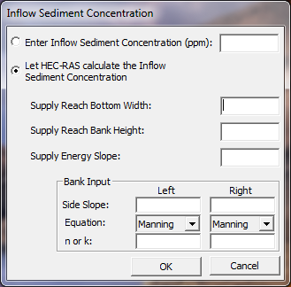
Figure 13 7. Inflow Sediment Concentration Window
Click OK to apply the input and return to the main HD Functions window. Once all of the required input has been entered, the Compute button will be activated. Click the Compute button to run the computations. When the computations are complete, the output table will be shown. The output table lists all of the channel widths solved for along with the corresponding depth, slope, composite n value, hydraulic radius, velocity, Froude number, shear stress and bed transport regime. An example is shown in Figure 13-8. There will be twenty different stable channel geometries plus one for the minimum stream power. The user can select one of these geometries for display on the plot window. Once the desired section is selected, click OK and the HD Functions window will become active with the selected section plotted in the plot window.
When the computations have been run, the Table button, the two Stability Curve buttons and the Copy to Geometry button become active. The Table button simply allows the user to pull up the output table again, and select a different stable section, if desired. Clicking on the Stability Curve 1 button will bring up a plot of the stability curve showing slope versus width, indicating for what slope/width combination aggradation or degradation can be expected. Figure 13-9 shows an example.
Figure 13 8. Copeland Method Output Table
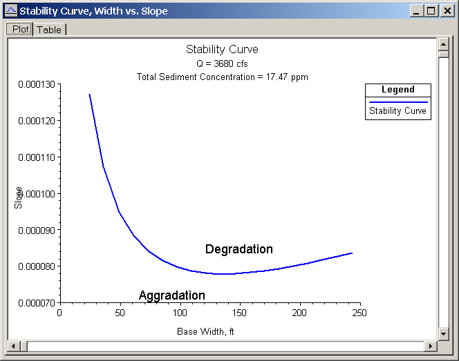
Figure 13 9. Stability Curve
Stability Curve 2 brings up a similar plot, only with slope compared to depth. In addition to viewing the plots, the table tab can be clicked to view the stability curves in tabular form.
As with the uniform flow computations, the section that has been plotted from the Copeland Method can be applied to the current geometry file by clicking on the Copy to Geometry button.
Brownlie is Limited to Sand Beds
The version of the Copeland Method currently in HEC-RAS only uses the Brownlie equations for transport and roughness. The Brownlie equations are limited to sand bed streams and designed for rivers with bedforms. The orriginal Copeland method also provided a MPM option for gravel bed streams. But the HEC-RAS method is limited to Brownlie and Sand Bed Streams.
Wish List - MPM Copeland Method
HEC would like to include the MPM version of the Copeland method for gravel bed streams.
Regime Method
To use the Regime Method, select the tab named "Regime." The window shown in Figure 13-10 becomes active.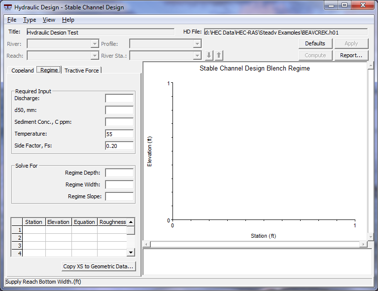
Figure 13 10. Regime Method
Enter in all required input which are:
Discharge: Channel forming discharge (cfs or m3/s).
d50: Median particle size (mm).
Sediment Conc, C ppm: The bed material sediment concentration, in ppm.
Temperature: A representative temperature of the water. Default is 55 degrees F or 10 degrees C.
Side Factor, Fs: The side factor as defined by Blench. Blench suggests 0.1 for friable banks, 0.2 for silty, clayey, or loamy banks, or 0.3 for tough clay banks. Default value is 0.2.
Once these values are entered, the compute button becomes activated and the stable channel regime values for depth, width, and slope will be solved for and entered into the appropriate fields. In addition, the plot window will display the resulting cross section.
The displayed cross section can be added to the existing geometry file by clicking on "Copy XS to Geometric Data."
Tractive Force Method
To use the Tractive Force Method, select the tab named "Tractive Force." The window shown in Figure 13-11 becomes active.
Figure 13 11. Tractive Force Method
Enter in all required input which are:
Discharge: Design discharge (cfs or m3/s).
Temperature: Temperature of the water. Default is 55 degrees F or 10 degrees C.
Specific Gravity: Specific gravity of the sediments for the left side slope, bed, and right side slope.
Angle of Repose: The angle of repose of the sediment for the left side slope, bed, and right side slope. See Figure 11-9 in the HEC-RAS Hydraulic Reference Manual for suggested values.
Side Slope: Left side slope and right side slope (1Vertical : __Horizontal).
Equation: the roughness equation for the left side slope, bed, and right side slope. Mannings and Strickler are available for use.
n or k: If Mannings is selected, enter a Mannings "n" value. If Strickler is selected, enter a "k" value for the left side slope, bed, and right side slope (ft or m for k values).
Method: Solve for critical shear using either Lane, Shields, or by entering in your own critical mobility parameter.
The remaining values are the dependant variables. Only two can be solved for at a time. The other two must be entered by the user. The three fields for particle diameter (left side slope, bed, right side slope) are considered one variable such that any one of the remaining variables plus any or all of the particle diameters can be solved for.
d50/d75: The particle diameter in which 50%/75% of the sediment is smaller, by weight. d50 is used for Shields and user-entered. d75 is used for Lane (mm).
D: The depth of the stable cross section (ft or m).
B: The bottom width of the stable cross section (ft or m).
S: The slope of the energy grade line at the stable cross section.
Once the required values plus two of the dependent variables are entered, the compute button becomes activated and the stable channel values for the remaining dependent variables will be solved for and entered into the appropriate fields. In addition, the plot window will display the resulting cross section.
The displayed cross section can be added to the existing geometry file by clicking on "Copy XS to Geometric Data."