Download PDF
Download page Boundary Conditions.
Boundary Conditions
There are several different types of boundary conditions available to the user. The following is a short discussion of each type:
Flow Hydrograph
A flow hydrograph can be used as either an upstream boundary or downstream boundary condition, but it is most commonly used as an upstream boundary condition. When the flow hydrograph button is pressed, the window shown in Figure 7-2 will appear. As shown, the user can either read the data from a HEC-DSS (HEC Data Storage System) file, or they can enter the hydrograph ordinates into a table. If the user selects the option to read the data from DSS, they must press the "Select DSS File and Path" button. When this button is pressed a DSS file and pathname selection screen will appear as shown in Figure 7-3. The user first selects the desired DSS file by using the browser button at the top. Once a DSS file is selected, a list of all of the DSS pathnames within that file will show up in the table. 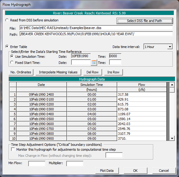
Figure 7 2. Example Flow Hydrograph Boundary Condition
The user also has the option of entering a flow hydrograph directly into a table, as shown in Figure 7-2. The first step is to enter a "Data time interval." Currently the program only supports regular interval time series data. A list of allowable time intervals is shown in the drop down window of the data interval list box. To enter data into the table, the user is required to select either "Use Simulation Time" or "Fixed Start Time." If the user selects "Use Simulation Time", then the hydrograph that they enter will always start at the beginning of the simulation time window. The simulation starting date and time is shown next to this box, but is grayed out. If the user selects "Fixed Start Time" then the hydrograph is entered starting at a user specified time and date. Once a starting date and time is selected, the user can then begin entering the data.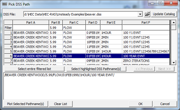
Figure 7 3. HEC-DSS File and Pathname Selection Screen
An option listed at the bottom of the flow hydrograph boundary condition is to make this boundary a "Critical Boundary Condition." When you select this option, the program will monitor the inflow hydrograph to see if a change in flow rate from one time step to the next is exceeded. If the change in flow rate does exceed the user entered maximum, the program will automatically cut the time step in half until the change in flow rate does not exceed the user specified max. Large changes in flow can cause instabilities. The use of this feature can help to keep the solution of the program stable. This feature can be used for multiple hydrographs simultaneously. The software will evaluate all of the hydrographs then calculate a time slice based on the hydrograph with the largest percentage increase over the user specified maximum flow change.
Two other options at the bottom of this editor are "Min Flow" and "Multiplier." Both of these options apply to user entered hydrographs or hydrographs read from HEC-DSS. The "Min Flow" option allows the user to specify a minimum flow to be used in the hydrograph. This option is very useful when too low of a flow is causing stability problems. Rather than edit the user entered hydrograph or the DSS file (depending upon where the hydrograph is coming from), the user can enter a single value, and all values below this magnitude will be changed to that value. The "Multiplier" option allows the user to multiply every ordinate of the hydrograph by a user specified factor. This factor will be applied to the user-entered hydrograph or a hydrograph read from HEC-DSS.
Stage Hydrograph
A stage hydrograph can be used as either an upstream or downstream boundary condition. The editor for a stage hydrograph is similar to the flow hydrograph editor (Figure 7-2). The user has the choice of either attaching a HEC-DSS file and pathname or entering the data directly into a table.
Stage and Flow Hydrograph
The stage and flow hydrograph option can be used together as either an upstream or downstream boundary condition. The upstream stage and flow hydrograph is a mixed boundary condition where the stage hydrograph is inserted as the upstream boundary until the stage hydrograph runs out of data; at this point the program automatically switches to using the flow hydrograph as the boundary condition. The end of the stage data is identified by the HEC-DSS missing data code of "-901.0". This type of boundary condition is primarily used for forecast models where the stage is observed data up to the time of forecast, and the flow data is a forecasted hydrograph.
Rating Curve
The rating curve option can be used as a downstream boundary condition. The user can either read the rating curve from HEC-DSS or enter it by hand into the editor. Shown in Figure 7-4 is the editor with data entered into the table. The downstream rating curve is a single valued relationship, and does not reflect a loop in the rating, which may occur during an event. This assumption may cause errors in the vicinity of the rating curve. The errors become a problem for streams with mild gradients where the slope of the water surface is not steep enough to dampen the errors over a relatively short distance. When using a rating curve, make sure that the rating curve is a sufficient distance downstream of the study area, such that any errors introduced by the rating curve do not affect the study reach.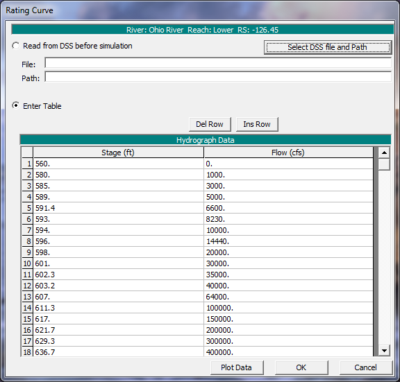
Figure 7 4. Example Rating Curve Boundary Condition Editor
Normal Depth
The Normal Depth option can only be used as a downstream boundary condition for an open-ended reach. This option uses Manning's equation to estimate a stage for each computed flow. To use this method the user is required to enter a friction slope (slope of the energy grade line) for the reach in the vicinity of the boundary condition. The slope of the water surface is often a good estimate of the friction slope, however this is hard to obtain ahead of time. The average bed slope in the vicinity of the boundary condition location is often used as an estimate for the friction slope.
As recommended with the rating curve option, when applying this type of boundary condition it should placed far enough downstream, such that any errors it produces will not affect the results at the study reach.
Lateral Inflow Hydrograph
The Lateral Inflow Hydrograph is used as an internal boundary condition. This option allows the user to bring in flow at a specific point along the stream. The user attaches this boundary condition to the river station of the cross section just upstream of where the lateral inflow will come in. The actual change in flow will not show up until the next cross section downstream from this inflow hydrograph. The user can either read the hydrograph from DSS or enter it by hand.
Uniform Lateral Inflow Hydrograph
The Uniform Lateral Inflow Hydrograph is used as an internal boundary condition. This option allows the user to bring in a flow hydrograph and distribute it uniformly along the river reach between two user specified cross section locations. The hydrograph for this boundary condition type can be either read in from DSS, or entered by hand into a table.
Groundwater Interflow
The groundwater boundary condition can be applied to a river reach or a storage area. Groundwater can flow into, or out of, a reach or storage area, depending on the water surface head. The stage of the groundwater reservoir is assumed to be independent of the interflow from the river, and must be entered manually or read from DSS. The groundwater interflow is similar to a uniform lateral inflow in that the user enters an upstream and a downstream river station, in which the flow passes back and forth. The groundwater interflow option can also be linked directly to a storage area, for modeling groundwater exchange with ponding areas. The computed flow is proportional to the head between the river (or storage area) and the groundwater reservoir.
The computation of the interflow is based on Darcy's equation. The user is required to enter the coefficient of permeability (hydraulic conductivity, K, in feet/day), a time series of stages for the groundwater aquifer, and the distance between the river and the location of the user entered groundwater aquifer stages (this is used to obtain a gradient for Darcy's equation). If the groundwater time-series represents the stage immediately at the cross section (for instance if the user has detailed results from a groundwater model), then the user should enter the "K of the streambed sediment" and the "Thickness of the streambed sediments." If the groundwater time-series is the stage some distance from the cross section (such as a monitoring well), then the user should enter an "Average K of the groundwater basin" and the "Distance between the river and the location of the groundwater stage."
Time Series of Gate Openings
This option allows the user to enter a time series of gate openings for an inline gated spillway, lateral gated spillway, or a gated spillway connecting two storage areas. The user has the option of reading the data from a DSS file or entering the data into a table from within the editor. Figure 7-5 shows an example of the Times Series of Gate Openings editor. As shown in Figure 7-5, the user first selects a gate group, then either attaches a DSS pathname to that group or enters the data into the table. This is done for each of the gate groups contained within the particular hydraulic structure.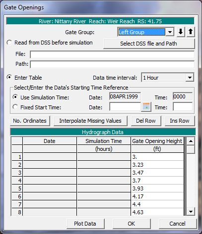
Figure 7 5. Example Time Series of Gate Openings Editor
Be Careful Opening or Closing Gates Too Quickly
Warning: Opening and closing gates too quickly can cause instabilities in the solution of the unsteady flow equations. If instabilities occur near gated locations, the user should either reduce the computational time step and/or reduce the rate at which gates are opened or closed.
Elevation Controlled Gate
This option allows the user to control the opening and closing of gates based on the elevation of the water surface upstream of the structure (Based on upstream WS); or based on the water surface at a user specified cross section or storage area (from any location in the model) (Based on specified reference); or based on a difference in water surface elevation from any two user defined reference locations (Based on difference in stage). A gate begins to open when a user specified elevation is exceeded. The gate opens at a rate specified by the user. As the water surface goes down, the gate will begin to close at a user specified elevation. The closing of the gate is at a user specified rate (feet/min.). If the gate operating criteria is a stage difference, the user can specify a stage difference for when the gate should open and a stage difference for when the gate should begin to close. Stage differences can be positive, zero, or negative values. The user must also enter a maximum and minimum gate opening, as well as the initial gate opening. Figure 7-6 shows an example of this editor.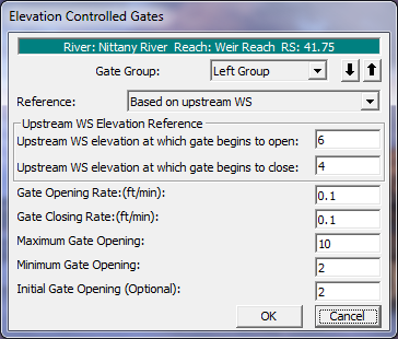
Figure 7 6. Elevation Controlled Gate Editor
Navigation Dam
This option allows the user to define an inline gated structure as a hinge pool operated navigation dam. The user specifies stage and flow monitoring locations, as well as a range of stages and flow factors. This data is used by the software to make decisions about gate operations in order to maintain water surface elevations at the monitor locations. A detailed discussion can be found in the Navigation Dams section.
Internal Boundary Stage and/or Flow Hydrograph
This option allows the user to enter a known stage hydrograph and/or a flow hydrograph, to be used as an internal boundary condition. The boundary condition can be used at a cross section immediately upstream of an inline structure in order to force a known stage and/or flow for part or all the simulation. It can also be used at an "open" cross section (one not associated with a hydraulic structure). For example, in order to force the water surface to match the water surface from known gage data. If the user enters only a stage hydrograph, then the program will force the stage at this cross section and it will solve for the appropriate flow (in order to balance the unsteady continuity and momentum equations). Similarly, if the user enters only a flow hydrograph, then the program will force the flow at this cross section and it will solve for the appropriate stage. The user may also enter both stage and flow data. In this case, the program will force the stage (and solve for flow) as long as there is stage data. Once the stage data runs out, the program will start using the flow data (force the flow and solve for stage). This can often be useful when performing a forecast. Regardless of whether a stage and/or flow hydrograph is entered, if all of the time series data runs out before the end of the simulation, then the program will treat the cross section as a regular cross section and will solve for both flow and stage in the normal manner.
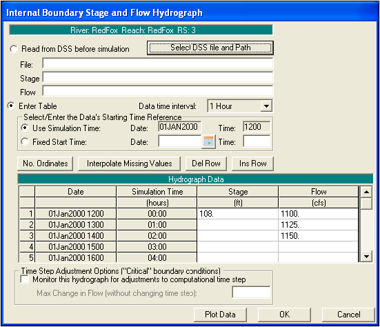
The Internal Boundary (IB) Stage and Flow Hydrograph editor is shown in Figure 7-7. In the example above, the program will force the stage to be 108 feet up until the start of the simulation time (that is, during the initial backwater and warm up period) and then it will start using the flow data. The flow for the first \[non-warm up\] time step will be 1100 cfs transitioning to 1125 cfs over the next hour. After two hours, the program will no longer force either stage or flow but, instead, will solve for both in a normal manner. Note: For an inline structure that has known discharges for all or part of the simulation, entering a single stage at the start of the simulation is a quick and easy way to enter an initial stage. (The alternative way to enter an initial stage is to go to the *Options* menu on the Unsteady Flow Data editor and select *Internal RS Stages…{*}) For the simulation in Figure 7-7, if the user had entered another stage, for example 107.5 feet at 01:00 hours, then the program would transition down to a stage of 107.5 feet during the first hour. At the start of the second hour, the flow would immediately be forced to a value of 1125 cfs. These sudden transitions may cause stability problems if the values are too far out of balance. For instance, if the program computed a flow value of 4400 cfs in order to force a water surface of 107.5 at the end of the first hour, then the system will receive a "shock" as the flow is forced to 1125 during the next time step. If a known hydrograph is entered for an inline structure (i.e. for the cross section immediately upstream of the inline structure) that has gates, then a boundary condition for the gate operations must still be entered (time series, elevation control, etc.). When the hydrograph information runs out, the program will use the gate operations from the boundary conditions and will solve for the flow and stage at the inline structure in a normal manner (computing weir and/or gate flow). As with the change from a stage hydrograph to a flow hydrograph, the change from known (stage or flow) hydrograph to normal inline operations can cause a "shock" if the new computed value is too far out of balance from the previous one. If the stage and/or flow hydrograph for a reservoir is entered for the entire simulation, then the physical characteristics of the inline structure will not affect the solution. In this situation, the inline structure does not even have to be entered into the geometry—the IB hydrograph could just be attached to an "open" cross section and the headwater and tailwater stages and flows would be the same. However, neither does it matter if the inline structure is included, and it may be convenient for display and/or output. If the user elects to use a DSS stage/flow hydrograph, then the "end of data" should be entered as a -901 in the DSS record, which is the missing data code for HEC-DSS. If the data is entered in the table, as shown in the example, then the end of data is a blank line. Do _not_ enter -901 in the table (unless this happens to be a real value).
"Rules" Editor
Currently HEC-RAS has the ability for the user to develop their own set of rules for controlling Inline structures, Lateral Structures, and Storage area Connections. The details of how the "Rules" editor can be used can be found in the User Defined Rules for Hydraulic Structures section.
Meteorological Data
HEC-RAS now has the capability to have spatially varying precipitation, wind, and infiltration. Spatial precipitation and wind data are added into the Unsteady Flow Boundary Conditions editor. While infiltration information is defined as a spatial layer in HEC-RAS Mapper.
Spatial precipitation and wind data can be entered into HEC-RAS as either gridded data or point gage data. The spatial precipitation/wind data is added into HEC-RAS through the Unsteady Flow Boundary Conditions editor. When that editor is open, you will find a tab on the main window called "Meteorological Data".
Precipitation
This option allows the user to enter a precipitation hyetograph to either a Storage Area or a 2D Flow Area. This option allows the user to enter incremental precipitation vs time via table entry or read in through HEC-DSS. Note, when hand entering precipitation in the table, the value entered for a given time should be the incremental precipitation over the previous period. The precipitation is used for the entire storage area or 2D flow area, with no spatial variability. If you want to use precipitation that is variable both spatially and in time, you can do that from the Meteorological Data Tab.
NOTE: To learn how to enter and use spatial precipitation and/or wind data with HEC-RAS, please review the section called "Global Boundary Conditions" in the 2D Modeling User's Manual here.