Download PDF
Download page Model Accuracy, Stability, and Sensitivity.
Model Accuracy, Stability, and Sensitivity
This section of the manual discusses model accuracy, stability, and sensitivity. In order to develop a good unsteady flow model of a river system, the user must understand how and why the solution of the unsteady flow equations becomes unstable. This knowledge will help you figure out why your particular model may be having stability problems. Additionally, it is important to understand the trade-offs between numerical accuracy (accurately solving the equations) and model stability. Finally, model sensitivity will be discussed in order to give you an understanding of what parameters affect the model and in what ways.
Model Accuracy
Model accuracy can be defined as the degree of closeness of the numerical solution to the true solution. Accuracy depends upon the following:
- Assumptions and limitations of the model (i.e. one dimensional model, single water surface across each cross section, etc…).
- Accuracy of the geometric Data (cross sections, Manning's n values, bridges, culverts, etc…).
- Accuracy of the flow data and boundary conditions (inflow hydrographs, rating curves, etc…).
- Numerical Accuracy of the solution scheme (solution of the unsteady flow equations).
Numerical Accuracy. If we assume that the 1-dimensional unsteady flow equations are a true representation of flow moving through a river system, then only an analytical solution of these equations will yield an exact solution. Finite difference solutions are approximate. An exact solution of the equations is not feasible for complex river systems, so HEC-RAS uses an implicit finite difference scheme.
Model Stability
An unstable numerical model is one for which certain types of numerical errors grow to the extent at which the solution begins to oscillate, or the errors become so large that the computations cannot continue. This is a common problem when working with an unsteady flow model of any size or complexity. Figure 7-40 is an example of a model that ran all the way through, but produced an unstable solution.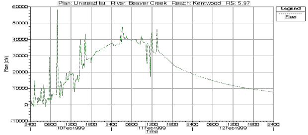
Figure 7 40. Hydrograph from an unstable solution.
The following factors will affect the stability and numerical accuracy of the model:
- Cross section spacing.
- Computation time step.
- Theta weighting factor for numerical solution.
- Calculation Options and Tolerances.
- Lateral Structures/Weirs
- Steep streams/mixed flow regime
- Downstream Boundary Conditions
- Cross section geometry and table properties
- Bridges and Culvert crossings
- Initial/low flow conditions
- Drops in bed profile.
- Manning's n values
- Missing or bad main channel data
For more information on how to identify and address these stability issues see the page on "Finding and Fixing Model Stability Problems"
Cross-Section Spacing
Cross sections should be placed at representative locations to describe the changes in geometry. Additional cross sections should be added at locations where changes occur in discharge, slope, velocity, and roughness. Cross sections must also be added at levees, bridges, culverts, and other structures.
Bed slope plays an important role in cross section spacing. Steeper slopes require more cross sections. Streams flowing at high velocities may require cross sections on the order of 100 feet or less. Larger uniform rivers with flat slopes may only require cross sections on the order of 5000 ft or more. However, most streams lie some where in between these two spacing distances.
Not enough cross sections: When cross sections are spaced far apart, and the changes in hydraulic properties are great, the solution can become unstable. In general, cross sections spaced too far apart will cause additional numerical diffusion, due to the derivatives with respect to distance being averaged over to long of a distance. Also, if the distance between cross sections is so great, such that the Courant number would be much smaller than 1.0, then the model may also become unstable. An example of varying cross section spacing is shown in Figure 7-41. Figure 7-41 shows an inflow hydrograph (dashed green line) and two outflow hydrographs (solid blue and black line with squares). As shown in the figure, as cross section spacing is increased, the hydrograph will show some numerical attenuation/diffusion.
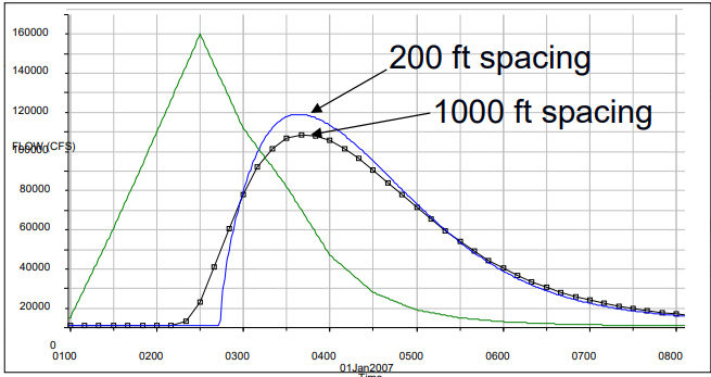
Figure 7 -41. The affects of cross section spacing on the hydrograph.
The general question about cross section spacing is "How do you know if you have enough cross sections." The easiest way to tell is to add additional cross sections (this can be done through the HEC-RAS cross section interpolation option) and save the geometry as a new file. Then make a new plan and execute the model, compare the two plans (with and without interpolated cross sections). If there are no significant differences between the results (profiles and hydrographs), then the original model without the additional cross sections is ok. If there are some significant differences, then additional cross sections should be gathered in the area where the differences occur. If it is not possible to get surveyed cross sections, or even cross sections from a GIS, then use the HEC-RAS interpolated cross sections. However, at least check the reasonableness of the interpolated cross sections with a topographic map. Edit any cross sections that do not look reasonable.
Cross Sections too Close. If the cross sections are too close together, then the derivatives with respect to distance may be overestimated (computed as steeper slopes than they should be), especially on the rising side of the flood wave. This can cause the leading edge of the flood wave to over steepen, to the point at which the model may become unstable. Figure 7-42 is an example where cross sections were placed very close together, and a very dynamic hydrograph was run through the river reach. The leading edge of the flood wave over steepened, and caused the model to produce an unstable result, which appears as a wall of water building just upstream of the flow going through critical depth. The solution to this problem is to remove some cross sections, which will allow the model to do a better job at computing the special derivatives.
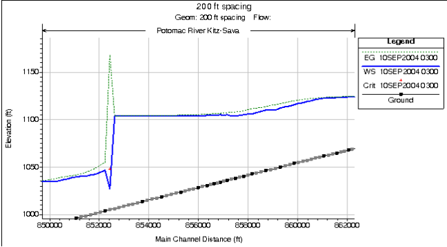
Figure 7 42. Stability problem from cross sections spaced to close together.
One of the first steps in stabilizing an unsteady flow model is to apply the correct cross section spacing. Dr. Danny Fread equation and P.G. Samuel's have developed equations for predicting maximum cross section spacing. These two equations are good starting points for estimating cross section spacing. Dr. Fread's equation is as follows:
\Delta x \le \frac {c*T_r} {20} |
where: Δx = Cross section spacing (ft)
Tr = Time of rise of the main flood wave (seconds)
c = Wave speed of the flood wave (ft/s)
Samuel's equation is as follows:
\Delta x \le \frac {0.15*D} {S_o} |
where: D = Average bank full depth of the main channel (ft)
So=Average bed slope (ft/ft)
Samuels equation is a little easier to use since you only have to estimate the average bank full depth and slope. For Fread's equation, although the time of rise of the hydrograph (Tr) is easy enough to determine, the wave speed (c) is a little more difficult to come by. At areas of extreme contraction and expansion, at grade breaks, or in abnormally steep reaches, inserting more cross sections may be necessary.
Computational Time Step
Stability and accuracy can be achieved by selecting a time step that satisfies the Courant Condition:
Cr = \frac{V_w*\Delta t}{\Delta x}\le 1.0 |
Therefore:
\Delta t \le \Delta x*\Delta V_w |
where: Vw = Flood wave speed, which is normally greater than the average velocity.
Cr = Courant Number. A value = 1.0 is optimal.
Δx=Distance between cross sections.
Δt=Computational time step.
For most rivers the flood wave speed can be calculated as:
V_w = \frac {dQ}{dA} |
However, an approximate way of calculating flood wave speed is to multiply the average velocity by a factor. Factors for various channel shapes are shown in the table below.
Table 7-2 Factors for Computing Wave Speed from Average Velocity
Ratio Vw/V | |
|---|---|
| Wide Rectangular | 1.67 |
| Wide Parabolic | 1.44 |
| Triangular | 1.33 |
| Natural Channel | 1.5 |
Too large of a time step: When the solution scheme solves the unsteady flow equations, derivatives are calculated with respect to distance and time. If the changes in hydraulic properties at a give cross section are changing rapidly with respect to time, the program may go unstable. The solution to this problem in general is to decrease the time step. An example of a hydrograph routed with two different time steps (1 minute and 10 minutes) is shown in Figure 7-43 below. As shown in the Figure, the hydrograph routed with a 10 minute time step has a much lower peak flow, and the leading edge of the floodwave is not as steep. This is due to the fact that the time based derivatives in the solution are averaging the changes in the floodwave over too long of a time step, thus numerically dampening the floodwave.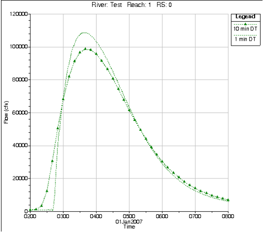
Figure 7 43. Hydrograph routed with two different time steps (1 and 10 minutes).
Too Small of a Time Step. If a time step is selected that is much smaller than what the Courant condition would dictate for a given flood wave, this can also cause model stability problems. In general to small of a time step will cause the leading edge of the flood wave to steepen, possible to the point of oscillating and going unstable.
Practical Time Step Selection
For medium to large rivers, the Courant condition may yield time steps that are too restrictive (i.e. a larger time step could be used and still maintain accuracy and stability). A practical time step is:
\Delta t \le \frac {T_r} {20} |
where: Tr=Time of rise of the hydrograph to be routed.
However, you may need to use a smaller time step when you have lateral weirs/spillways and hydraulic connections between storage areas and the river system. Also, if you are opening and closing gates quickly, or modeling a Dam or Levee breach, you will need to use very small time steps (less than a minute, maybe even as low as 5 seconds).
Theta Weighting Factor
Theta is a weighting applied to the finite difference approximations when solving the unsteady flow equations. Theoretically Theta can vary from 0.5 to 1.0. However, a practical limit is from 0.6 to 1.0 Theta of 1.0 provides the most stability, but less numerical accuracy. Theta of 0.6 provides the most accuracy, but less numerical stability. The default in HEC-RAS is 1.0. Once you have your model developed, reduce theta towards 0.6, as long as the model stays stable.
Larger values of theta increase numerical diffusion, but by how much? Experience has shown that for short period waves that rapidly rise, theta of 1.0 can produce significant errors. However, errors in the solution can be reduced by using smaller time steps.
When choosing theta, one must balance accuracy and computational robustness. Larger values of theta produce a solution that is more robust, less prone to blowing up. Smaller values of theta, while more accurate, tend to cause oscillations in the solution, which are amplified if there are large numbers of internal boundary conditions. Test the sensitivity of theta to your data set. If reducing theta does not change the solution, then the larger value should be used to insure greater stability.
For rivers with tidal boundaries, in which the rising tide will propagate upstream, the user should always try to use a theta value as close to 0.6 as possible. Tidal waves are very dynamic. In order for the solution to be able to accurately model a tidal surge, theta must be close to 0.6.
Calculation Options and Tolerances
Within the HEC-RAS software there are several calculation options and tolerances that can affect the stability and accuracy of the solution. Some of the more important calculation options and tolerances are:
Calculation Tolerances: Three solution tolerances can be set or changed by the user: Water surface calculation (0.02 default); Storage area elevation (0.02 default); and Flow calculation (Default is that it is not used). The default values should be good for most river systems. Only change them if you are sure!!!
Making the tolerances larger will actually make the mode less stable. Making the tolerances smaller will make the model more stable, but may cause the program to iterate more, thus increasing the run time.
Maximum Number of Iterations: At each time step derivatives are estimated and the equations are solved. All of the computation nodes are then checked for numerical error. If the error is greater than the allowable tolerances, the program will iterate. The default number of iterations in HEC-RAS is set to 20. Iteration will generally improve the solution. This is especially true when your model has lateral weirs and storage areas.
Warm up time step and duration: The user can instruct the program to run a number of iterations at the beginning of the simulation in which all inflows are held constant. This is called the warm up period. The default is not to perform a warm up period, but the user can specify a number of time steps to use for the warm up period. The user can also specify a specific time step to use (default is to use the user selected computation interval). The warm up period does not advance the simulation in time, it is generally used to allow the unsteady flow equations to establish a stable flow and stage before proceeding with the computations.
Time Slicing: The user can control the maximum number of time slices and the minimum time step used during time slicing. There are two ways to invoke time slicing: rate of change of an inflow hydrograph or when a maximum number of iterations is reached.
At each time step derivatives are estimated and the equations are solved. All of the computation nodes are then checked for numerical error. If the error is greater than the allowable tolerances, the program will iterate. The default number of iterations in HEC-RAS is set to 20. Iteration will generally improve the solution. This is especially true when your model has lateral weirs and storage areas.
Inline and Lateral Structure Stability Issues
Inline and Lateral Structures can often be a source of instability in the solution. Especially lateral structures, which take flow away or bring it into the main river. During each time step, the flow over a weir/spillway is assumed to be constant. This can cause oscillations by sending too much flow during a time step. One solution is to reduce the time step. Another solution is to use Inline and Lateral Structure stability factors, which can smooth these oscillations by damping the initial estimate of the computed flows.
The Inline and Lateral Structure stability factors can range from 1.0 to 3.0. The default value of 1.0 is essentially no damping of the computed flows. As you increase the factor you get greater dampening of the initial guess of the flows (which will provide for greater stability).
Long and flat Lateral Weirs/Spillways
during the computations there will be a point at which for one time step no flow is going over the lateral weir, and then the very next time step there is. If the water surface is rising rapidly, and the weir is wide and flat, the first time the water surface goes above the weir could result in a very large flow being computed (i.e. it does not take a large depth above the weir to produce are large flow if it is very wide and flat). This can result in a great decrease in stage from the main river, which in turn causes the solution to oscillate and possible go unstable. This is also a common problem when having large flat weirs between storage areas. The solution to this problem is to use smaller computational time steps, and/or weir/spillway stability factors.
Opening gated spillways to quickly
When you have a gated structure in the system, and you open it quickly, if the flow coming out of that structure is a significant percentage of the flow in the receiving body of water, then the resulting stage, area and velocity will increase very quickly. This abrupt change in the hydraulic properties can lead to instabilities in the solution. To solve this problem you should use smaller computational time steps, or open the gate a littler slower, or both if necessary
Weir and Gated Spillway Submergence Factors.
When you have a weir or gated spillway connecting two storage areas, or a storage area and a reach, oscillations can occur when the weir or gated spillway becomes highly submerged. The program must always have flow going one way or the other when the water surface is above the weir/spillway. When a weir/spillway is highly submerged, the amount of flow can vary greatly with small changes in stage on one side or the other. This is due to the fact that the submergence curves, which are used to reduce the flow as it becomes more submerged, are very steep in the range of 95 to 100 percent submergence. The net effect of this is that you can get oscillations in the flow and stage hydrograph when you get to very high submergence levels. The program will calculate a flow in one direction at one time step. That flow may increase the stage on the receiving side of the weir, so the next time step it sends flow in the other direction. This type of oscillation is ok if it is small in magnitude. However, if the oscillations grow, they can cause the program to go unstable.
To reduce the oscillations, the user can increase the Weir/Spillway Submergence Factor. This factor can vary from 1.0 to 3.0. A factor of 1.0 leaves the submergence criteria in its original form. Using a factor greater than 1.0 causes the program to use larger submergence factors earlier, and makes the submergence curve less steep at high degrees of submergence. A plot of the submergence curves for various factors is shown in Figure 7-44.
The net result of using a weir flow submergence factor greater than 1.0, is the flow rate will be reduced more at lower degrees of submergence, but the computations will be much more stable at high degrees of submergence.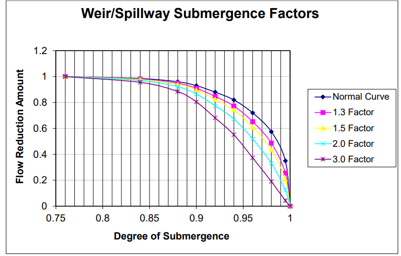 Figure 7 44. Weir/Spillway Submergence Factors.
Steep Streams and Mixed Flow Regime
Higher velocities and rapid changes in depth and velocity are more difficult to model and keep a stable solution. As the Froude number approaches 1.0 (critical depth), the inertial terms of the St. Venant equations and their associated derivatives tend to cause model instabilities (For the 1D Finite Difference solver). The default solution methodology for unsteady flow routing within HEC-RAS is generally for subcritcal flow. The software does have an option to run in a mixed flow regime mode. However, this option should not be used unless you truly believe you have a mixed flow regime river system. If you are running the software in the default mode (subcritical only, no mixed flow), and if the program goes down to critical depth at a cross section, the changes in area, depth, and velocity are very high. This sharp increase in the water surface slope will often cause the program to overestimate the depth at the next cross section upstream, and possible underestimate the depth at the next cross section downstream (or even the one that went to critical depth the previous time step). One solution to this problem is to increase the Manning's n value in the area where the program is first going to critical depth. This will force the solution to a subcritical answer and allow it to continue with the run. If you feel that the true water surface should go to critical depth, or even to a supercritical flow regime, then the mixed flow regime option should be turned on. Another solution is to increase the base flow in the hydrographs, as well as the base flows used for computing the initial conditions. Increased base flow will often dampen out any water surfaces going towards or through critical depth due to low flows.
Bad downstream boundary condition
If the user entered downstream boundary condition causes abrupt jumps in the water surface, or water surface elevations that are too low (approaching or going below critical depth), this can cause oscillations in the solution that may lead to it going unstable and stopping. Examples of this are rating curves with not enough points or just simply too low of stages; and normal depth boundary conditions where the user has entered too steep of a slope. Shown in Figure 7-45 is an example in which a Normal depth boundary condition was used with too steep of an energy slope entered by the user. The net affect was that for any given flow, the water surface elevation was computed much lower than it should have been, as shown in the figure. The water surface just upstream of the boundary condition becomes very steep, and potentially can lead to an unstable solution.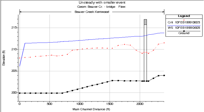
Figure 7 45. Example of a bad downstream boundary condition.
Cross section Geometry and Table properties
All of the cross sections get converted to tables of hydraulic properties (elevation versus area, conveyance, and storage). If the curves that represent these hydraulic properties have abrupt changes with small changes in elevation, this can also lead to instability problems. This situation is commonly caused by: levees being overtopped with large areas behind them (since the model is one dimensional, it assumes that the water surface is the same all the way across the entire cross section); and ineffective flow areas with large amounts of storage that are turned on at one elevation, and then turn off at a slightly higher elevation (this makes the entire area now used as active conveyance area). There are many possible solutions to these problems, but the basic solution is to not allow the hydraulic properties of a cross section to change so abruptly. If you have a levee with a large amount of area behind it, model the area behind the levee separately from the cross section. This can be done with either a storage area or another routing reach, whichever is most hydraulically correct for the flow going over the levee or if the levee breaches. With large ineffective flow areas, the possible solutions are to model them as being permanently on, or to put very high Manning's n values in the ineffective zones. Permanent ineffective flow areas allow water to convey over top of the ineffective area, so the change in conveyance and area is small. The use of high Manning's n values reduces the abruptness in the change in area and conveyance when the ineffective flow area gets turned off and starts conveying water.
Cross section property tables that do not go high enough: The program creates tables of elevation versus area, conveyance, and storage area for each of the cross sections. These tables are used during the unsteady flow solution to make the calculations much faster. By default, the program will create tables that extend up to the highest point in the cross section, however, the user can override this and specify their own table properties (increment and number of points). If during the solution the water surface goes above the highest elevation in the table, the program simply extrapolates the hydraulic properties from the last two points in the table. This can lead to bad water surface elevations or even instabilities in the solution.
Not enough definition in cross section property tables: The counter problem to the previous paragraph is when the cross section properties in a given table are spread too far apart, and do not adequately define the changes in the hydraulic properties. Because the program uses straight-line interpolation between the points, this can lead to inaccurate solutions or even instabilities. To reduce this problem, we have increased the allowable number of points in the tables to 100. With this number of points, this problem should not happen.
Bridge and Culvert crossings
Bridge/Culvert crossings can be a common source of model stability problems when performing an unsteady flow analysis. Bridges may be overtopped during an event, or even washed out. Common problems at bridges/culverts are the extreme rapid rise in stages when flow hits the low chord of the bridge deck or the top of the culvert. Modelers need to check the computed curves closely and make sure they are reasonable. One solution to this problem is to use smaller time steps, such that the rate of rise in the water surface is smaller for a given time step. Modelers may also need to change hydraulic coefficients to get curves that have more reasonable transitions.
An additional problem is when the curves do not go high enough, and the program extrapolates from the last two points in the curve. This extrapolation can cause problems when it is not consistent with the cross section geometry upstream and downstream of the structure.
For bridge and culvert crossing the program creates a family of rating curves to define all the possible headwater, tailwater, and flow combinations that can occur at a particular structure. One free flow curve (headwater versus flow, with no influence from the tailwater) is calculated with fifty points to define it, then up to fifty submerged curves (headwater versus flow, staring at a particular tailwater) are calculated with up to 20 points to define each curve. The user can control how many submerged curves get calculated, how many points in each curve, and the properties used to define the limits of the curves (maximum headwater, maximum tailwater, maximum flow, and maximum head difference). By default, the software will take the curves up to an elevation equal to the highest point in the cross section just upstream of the structure. This may lead to curves that are too spread out and go up to a flow rate that is way beyond anything realistic for that structure. These type of problems can be reduced by entering specific table limits for maximum headwater, tailwater, flow, and head difference. An example set of curves are shown in Figure 7-46.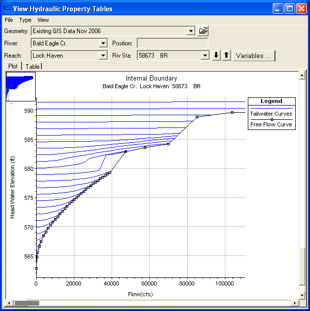 Figure 7 46. Example Family of Curves for a Bridge crossing.
Ineffective flow areas are required up and downstream of bridges and culverts to properly define the contraction and expansion zones. Unsteady flow models, and particularly dam breach models, need these zones to be adequately defined. When the bridge is overtopped, the ineffective flow areas will turn off. This sudden and large increase in conveyance can cause model instability. One solution is to use very high Manning's n values (.2 to 1.0) in the ineffective flow zones, so when they turn off the increase in conveyance is not so great. This is also more physically appropriate as the cross sections just upstream and downstream can not flow completely freely because of the bridge embankment.
Initial Conditions and Low Flow
When starting a simulation it is very common to start the system at low flows. Make sure that the initial conditions flow is consistent with the first time step flow from the unsteady flow boundary conditions. User's must also pay close attention to initial gate settings and flows coming out of a reservoir, as well as the initial stage of the pool in the reservoir. The initial condition flow values must be consistent with all inflow hydrographs, as well as the initial flows coming out of the reservoir.
Flows entered on the initial conditions tab of the Unsteady Flow Data editor are used for calculating stages in the river system based on steady flow backwater calculations. If these flows and stages are inconsistent with the initial flows in the hydrographs, and coming out of the reservoir, then the model may have computational stability problems at the very beginning of the unsteady flow computations.
If any portion of an inflow hydrograph is so low that it causes the stream to go through a pool and riffle sequence, it may be necessary to increase the base flow. The minimum flow value must be small enough that it is negligible when compared to the peak of the flood wave. A good rule of thumb is to start with a minimum flow equal to about 1 % of the peak flood (inflow hydrograph, or dam breach flood wave) and increase as necessary to 10%. If more than 10% is needed, then the problem is probably from something else.
If you have some cross sections that are fairly wide, the depth will be very small. As flow begins to come into the river, the water surface will change quickly. The leading edge of the flood wave will have a very steep slope. Sometimes this steep slope will cause the solution to reduce the depth even further downstream of the rise in the water surface, possibly even producing a negative depth. This is due to the fact that the steep slope gets projected to the next cross section downstream when trying to solve for its water surface. The best solution to this problem is to use what is called a pilot channel. A pilot channel is a small slot at the bottom of the cross section, which gives the cross section a greater depth without adding much flow area. This allows the program to compute shallow depths on the leading edge of the flood wave without going unstable. Another solution to this problem is to use a larger base flow at the beginning of the simulation.
Drops in the Bed Profile
Significant drops in the bed profile can also be a source of model stability problems, especially at low flows. If the drop is very small, then usually an increase in baseflow will drowned out the drop, thus preventing the model from passing through critical depth. If the drop is significant, then it should be modeled with an inline structure using a weir. This will allow the model to use a weir equation for calculating the upstream water surface for a given flow, rather than using the unsteady flow equations. This produces a much more stable model, as the program does not have to model the flow passing through critical depth with the unsteady flow equations. HEC-RAS automatically handles submergence on the weir, so this is not a problem. An example of a profile drop that causes a model stability problem is shown in Figure 7-47.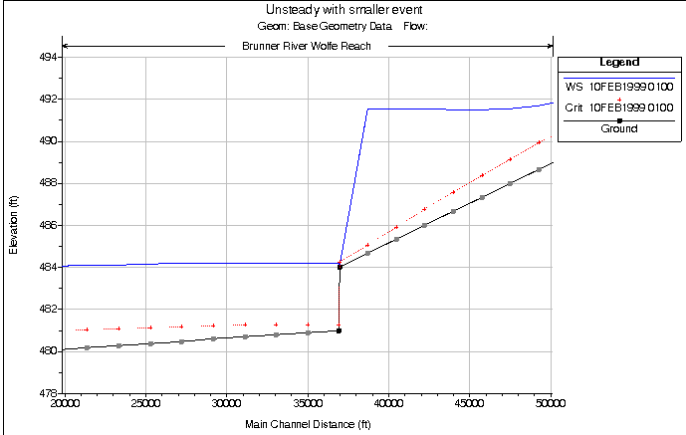
Figure 7 47. Stability Problem caused by drop in bed profile.
When an Inline Structure (weir) is added to the above data set, the model is able to obtain a stable and accurate solution of the profile (Figure 7-48).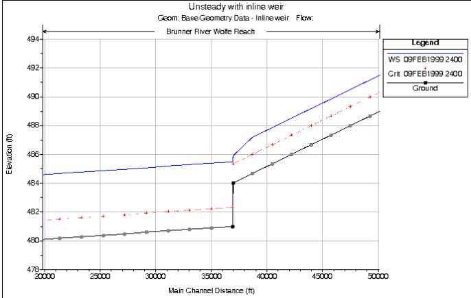
Figure 7 48. Stable solution using Inline Structure to represent profile drop.
Some additional solutions to the problem of significant drops in the channel invert are: increase the base flow to a high enough value to drowned out the drop in the bed profile; put a rating curve into the cross section at the top of the drop (this will prevent the unsteady flow equations being solved through the drop, the rating curve will be used instead); and add more cross section, if the drop is gradual, and run the program in mixed flow regime mode.
Manning's n Values
Manning's n values can also be a source of model instability. Manning's n values that are too low, will cause shallower depths of water, higher velocities, and possibly even supercritical flows. This is especially critical in steep streams, where the velocities will already be high. User's should check there estimated Manning's n values closely in order to ensure reasonable values. It is very common to underestimate Manning's n values in steep streams. Use Dr. Robert Jarrets equation for steep streams to check your main channel Manning's n values. An example model stability problem due to too low on Manning's n values being used in steep reaches is shown in Figure 7-49.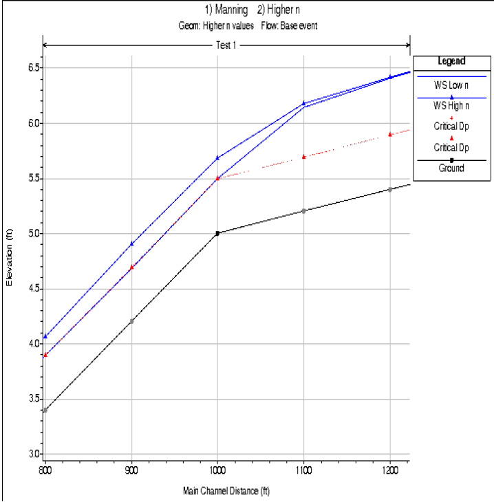
Figure 7 49. Model stability problem due to low Manning's n values.
Over-estimating Manning's n values will cause higher stages and more hydrograph attenuation than may be realistic.
Missing or Bad Channel Data
Another typical source of instabilities occurs when the main channel has a wide flat bed. This is usually found when cross sections are approximated or when terrain data is used to develop cross sections exclusive of real bathymetric data. Many times reaches are developed in GIS using LIDAR data or other aerial means. These survey methods don't penetrate water surfaces so the main channel is left with a flat horizontal bed equal to the water surface elevation (Figure 7-50). For dam breach analyses, shallow streams are normally okay, since the dam break flood wave is usually much greater than the depth of water in the channel. However, wide flat stream beds tend to cause instabilities because at lower flows, the area to depth ratio is very high. When this occurs, a small increase in depth is seen as a large relative increase in depth.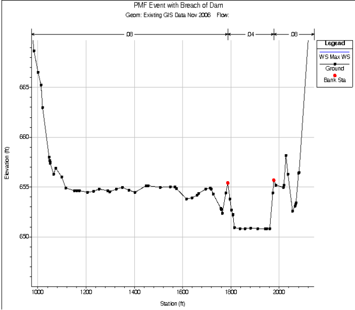 Figure 7 50. Example Cross Section missing most of the main channel.
Additionally, in the cross section plot, if high ground that is not appropriately accounted for can be a source of instabilities. High ground can be modeled as levees or with ineffective flows to remove the abrupt changes in storage and conveyance when the high ground is overtopped.
Stream Junction Issues
The unsteady flow equation solver, by default, makes a simplifying assumption at stream junctions. The unsteady solver forces the same exact water surface at all cross sections that bound a junction (Upstream and downstream of the junction). This simplifying assumption is fine for flat to moderately sloping streams. However, once you get to medium to steep sloping streams, this is normally a bad assumption, and can even cause model instability issues.
In general, cross sections placed around stream junctions should be placed as close to the junction as possible, such that the assumption of equal water surface elevation is not so bad. Sometimes this is not possible. For example, in steep streams, the first cross section of a tributary coming into a main stem may have a higher channel invert than the main stem river. If you are starting the model at a low flow, the program computes the water surface in the main river below the junction, then forces that water surface on the cross sections upstream of the junction, both in the main river and the tributary. This can often end up with way too low of a water surface elevation in the tributary, for the given flow rate, which very quickly causes the model to go unstable in the tributary reach near the junction.
The solution to this problem, is to first ensure you have the cross sections bounding the junction, as close to the junction as possible. Second, compare at the main channel elevations of all the cross sections that bound the junction. If one cross section is much higher than the others (say the tributary one), then there will be a problem trying to run this model at low flow. Either extract a new cross section closer to the junction (thus having a lower main channel), or adjust the main channel data of that cross section.
An additional option that has been added to HEC-RAS to assist in this problem, is the option to use an "Energy Balance Method" to compute the water surface elevations across the junction during the unsteady flow computations. This option will allow for sloping water surface elevations across the junction and can help alleviate many model stability issues at junctions in medium to steep sloping streams.
Model Sensitivity
Model sensitivity is an important part of understanding the accuracy and uncertainty of the model. There are two types of sensitivity analysis that should be performed, Numerical Sensitivity and Physical Parameter Sensitivity.
Numerical Sensitivity
Numerical Sensitivity is the process of adjusting parameters that affect the numerical solution in order to obtain the best solution to the equations, while still maintaining model stability. The following parameters are typically adjusted for this type of sensitivity analysis:
Computational Time Step - The user should try a smaller time step to see if the results change significantly. If the results do change significantly, then the original time step is probably too large to solve the problem accurately.
Theta Weighting Factor - The default value for this factor is 1.0, which provides the greatest amount of stability for the solution, but may reduce the accuracy. After the user has a working model, this factor should be reduced towards 0.6 to see if the results change. If the results do change, then the new value should be used, as long as the model stays stable. Be aware that using a value of 0.6 gives the greatest accuracy in the solution of the equations, but it may open the solution up to stability problems.
Weir/Spillway Stability Factors – If you are using these factors to maintain stability, try to reduce them to the lowest value you can and still maintain stability. The default value is 1.0, which is no stability damping.
Weir/Spillway Submergence Exponents – In general these parameters will not affect the answers significantly, they only provide greater stability when a spillway/weir is at a very high submergence. Try reducing them towards 1.0 (which is no factor) to see if the model will remain stable.
Physical Parameter Sensitivity
Physical Parameter Sensitivity is the process of adjusting hydraulic parameters and geometric properties in order to test the uncertainty of the models solutions. This type of sensitivity analysis is often done to gain an understanding of the possible range of solutions, given realistic changes in the model parameters. Another application of this type of sensitivity analysis is to quantify the uncertainty in the model results for a range of statistical events (2, 5,10, 25, 50, 100 yr, etc…). The following data are often adjusted during this type of sensitivity analysis:
Manning's n Values – Manning's n values are estimated from physical data about the stream and floodplain. Sometimes Manning's n values are calibrated for a limited number of events. Either way, the values are not exact! The modeler should estimate a realistic range that the n values could be for their stream. For example, if you estimated an n value for a stream as 0.035, a realistic range for this might be 0.03 to 0.045. The modeler should run the lower Manning's n values and the higher Manning's n values to evaluate their sensitivity to the final model results.
Cross Section Spacing – Cross section spacing should always be tested to ensure that you have enough cross sections to accurately describe the water surface profiles. One way to test if you have enough cross sections is to use the HEC-RAS cross section interpolation routine, and interpolate enough cross sections to cut the average distance between cross sections in half. Re-run the model, if the results have not changed significantly, then your original model was probably fine. If the results do change significantly, then you should either get more surveyed cross sections or use the interpolated cross sections. If you use the interpolated cross sections, then you should at least look at a topographic map to ensure that the interpolated cross sections are reasonable. If the interpolated cross sections are not reasonable in a specific area, then simply edit them directly to reflect what is reasonable based on the topographic map.
Cross Section Storage – Portions of cross sections are often defined with ineffective flow areas, which represents water that has no conveyance. The extent of the storage within a cross section is an estimate. What if the ineffective flow areas were larger or smaller? How would this effect the results? This is another area that should be tested to see the sensitivity to the final solution.
Lateral Weir/Spillway Coefficients – Lateral weir/spillway coefficients can have a great impact on the results of a simulation, because they take water away or bring water into the main stream system. These coefficients can vary greatly for a lateral structure, depending upon their angle to the main flow, the velocity of the main flow, and other factors. The sensitivity of these coefficients should also be evaluated.
Bridge/Culvert Parameters – In general, bridge and culvert parameters normally only effect the locally computed water surface elevations just upstream and downstream of the structure. The effect that a bridge or culvert structure will have on the water surface is much greater in flat streams (a small increase in water surface can back upstream for a long distance if the river is flat). However, the sensitivity of the water surface elevations around a bridge or culvert may be very important to localized flooding. The bridge and culvert hydraulic parameters should also be evaluated to test their sensitivity.