Download page Finding and Fixing Model Stability Problems.
Finding and Fixing Model Stability Problems
Detecting Model Stability Problems. One of the hardest things about using an unsteady flow model is to get the model to be stable, as well as accurate, for the range of events to be modeled. When you first start putting together an unsteady flow model, undoubtedly you will run in to some stability problems. The question is, how do you know you are having a stability problem? The following is a list of stability problem indicators:
Program stops running during the simulation with a math error, or states that the matrix solution went unstable.
Program goes to the maximum number of iterations for several time steps in a row with large numerical errors.
There are unrealistic oscillations in the computed stage and flow hydrographs, or the water surface profiles.
The computed error in the water surface elevation is very large.
What do you do when this happens?
Note the simulation time and location from the computation window when the program either blew up or first started to go to the maximum number of iterations with large water surface errors.
Use the HEC-RAS Profile and Cross Section Plots as well as the Tabular Output to find the problem location and issue.
If you cannot find the problem using the normal HEC-RAS output - Turn on the "Computation Level Output" option and re-run the program.
View the time series and profile output associated with the Computation Level Output option. Locate the simulation output at the simulation time when the solution first started to go bad.
Find the river station locations that did not meet the solution tolerances. Then check the data in this general area.
The Computational Window is the first place to look for problems. When the maximum number of iterations is reach, and solution error is greater than the predefined tolerance, the time step, river, reach, river station, water surface elevation and the amount of error is reported. When the error increases too much, the solution will stop and say "Matrix Solution Failed". Often the first river station to show up on the window can give clues to the source of instabilities.
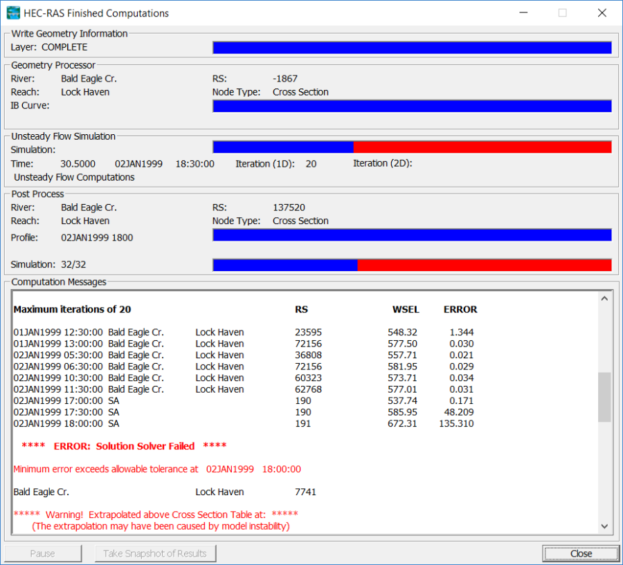
An example of the Computation Window with an unstable model solution is shown in Figure 7-51.
Figure 751. Example Unsteady Flow Computation window with unstable solution.
The first place to look for instabilities and errors is the Computations Window during and just after the simulation is run. The red progress bar indicates the model went unstable and could not complete the simulation. The Computation Messages window provides a running dialog of what is happening in the simulation at a given time step in a given location. This allows the user to watch errors propagate during the simulation. Once the simulation has crashed, don't close the Computations Window. Instead, scroll up through the messages and try to determine where the propagation of errors began, and at what time.
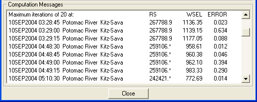
Sometimes the first error to occur is at the beginning of the simulation and is just a result of the model settling out after the transition from initial conditions to the first time step. Particularly if the error only occurs once for that given river station. It is better to focus on reoccurring errors or compounding errors first. The example shown in Figure 7-52 shows a relatively small error at river station 259106* that grows to 0.4 ft in the next few time steps. Figure 752. Example of growing computational errors.