Download PDF
Download page Performing a Steady Flow Analysis.
Performing a Steady Flow Analysis
This chapter discusses how to calculate steady flow water surface profiles. The chapter is divided into two parts. The first part discusses how to enter steady flow data and boundary conditions. The second part discusses how to develop a plan and perform the calculations.
Entering and Editing Steady Flow Data
Once all of the geometric data are entered, the modeler can then enter any steady flow data that are required. To bring up the steady flow data editor, select Steady Flow Data from the Edit menu on the HEC-RAS main window. The steady flow data editor should appear as below.
The user is required to enter the following information: the number of profiles to be calculated; the peak flow data (at least one flow for every river reach and every profile); and any required boundary conditions. The user should enter the number of profiles first. The next step is to enter the flow data. Flow data are entered directly into the table. Use the mouse pointer to select the box in which to enter the flow then type in the desired value.
Flow data are entered from upstream to downstream for each reach. At least one flow value must be entered for each reach in the river system. Once a flow value is entered at the upstream end of a reach, it is assumed that the flow remains constant until another flow value is encountered within the reach. The flow data can be changed at any cross section within a reach. To add a flow change location to the table, first select the reach in which you would like to change the flow (from the river and reach boxes above the table). Next, select the River Station location for which you want to enter a flow change. Then press the Add Flow Change Location button. The new flow change location will appear in the table. If the user wants to add multiple flow change locations, select the button labeled Add Multiple. This will bring up a window that will allow the user to select multiple locations all at one time.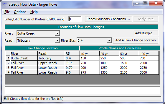
Each profile is automatically assigned a title based on the profile number, such as profile #1 is assigned a title of "Prof #1," profile #2 is assigned a title of "Prof #2," etc. The user can rename the title for each profile by simply going into the options menu and selecting Edit Profile Names. Once this option is selected, a dialog will appear allowing you to rename each of the profile titles.
Steady Flow Data Options
Several options are available from the steady flow data editor to assist users in entering the data. These features can be found under the Options menu at the top of the window. The following options are available:
Undo Editing. This option allows the user to retrieve the data back to the form that it was in the last time the Apply Data button was pressed. Each time the Apply Data button is pressed, the Undo Editing feature is reset to the current information.
Copy Table to Clipboard (with headers). This option allows the user to copy all of the reach, river, river station, and corresponding flow data to the clipboard. This can be very useful if you want to manipulate the data outside of HEC-RAS, such as in Excel.
Delete Row From Table. This option allows the user to delete a row from the flow data table. To use this option, first select the row to be deleted with the mouse pointer. Then select Delete Row From Table from the options menu. The row will be deleted and all rows below it will move up one.
Delete All Rows From Table. This option allows the user to delete all of the rows from the table. To use this option, select Delete All Rows From Table from the Options menu. When this option is selected a window will appear with a question to make sure that deleting all of the row is what you really want to do.
Delete Column (Profile) From Table. This option allows the user to delete a specific column (profile) of data from the table. To use this option, first select the column that you want to delete by placing the mouse over any cell of that column and clicking the left mouse button. Then select Delete Column (Profile) From Table from the Options menus. The desired column will then be deleted.
Ratio Selected Flows. This option allows the user to multiply selected values in the table by a factor. Using the mouse pointer, hold down the left mouse button and highlight the cells that you would like to change by a factor. Next, select Ratio Selected Flows from the options menu. A pop up window will appear allowing you to enter a factor to multiply the flows by. Once you press the OK button, the highlighted cells will be updated with the new values.
Edit Profile Names. This option allows the user to change the profile names from the defaults of PF#1, PF#2, etc.
Set Changes in WS and EG. This option allows the user to set specific changes in the water surface and energy between any two cross sections in the model. The changes in water surface and energy can be set for a specific profile in a multiple profile model. When this option is selected, a window will appear as shown in Figure 6-3. As shown, there are five options that the user can select from: Additional EG, Change in EG, Known WS, Change in WS, and K Loss. The Additional EG option allows the user to add an additional energy loss between two cross sections. This energy loss will be used in the energy balance equation in addition to the normal friction and contraction and expansion losses. The Change in EG option allows the user to set a specific amount of energy loss between two cross sections. When this option is selected, the program does not perform an energy balance, it simply adds the specified energy loss to the energy of the downstream section and computes a corresponding water surface. The Known WS option allows the user to set a water surface at a specific cross section for a specific profile. During the computations, the program will not compute a water surface elevation for any cross section where a known water surface elevation has been entered. The program will use the known water surface elevation and then move to the next section. The Change in WS option allows the user to force a specific change in the water surface elevation between two cross sections. When this option is selected, the program adds the user specified change in water surface to the downstream cross section, and then calculates a corresponding energy to match the new water surface. The K Loss option allows the user to calculate an additional energy loss that will be added into the solution of the energy balance. This energy loss is calculated by taking the user entered K coefficient, times the velocity head at the current cross section being solved. The user entered K coefficient can range from 0.0 to 1.0. The K value is very analogous to a minor loss coefficient, as found in pipe flow hydraulics.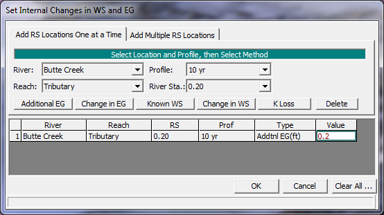
As shown in the figure above, to use the "Set Internal Changes in WS and EG" option, the user first selects the river, reach, river station, and profile that they would like to add an internal change too. Once the user has established a location and profile, the next step is to select one of the five available options by pressing the appropriate button. Once one of the five buttons are pressed, a row will be added to the table at the bottom, and the user can then enter a number in the value column, which represents the magnitude of the internal change or required coefficient.
Observed WS. This option allows the user to enter observed water surfaces at any cross section for any of the computed profiles. The observed water surfaces can be displayed on the profile plots, cross section plots, and in the summary output tables. To use this option select Observed WS from the Options menu.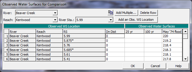
As shown in figure above, the user selected a River, Reach, and River Station location, then press the Add an Obs. WS Location (or Add Multiple) to enter a row in the table. Then enter the observed water surface for any of the profiles that are applicable. The column in the table labeled Dn Dist can be used to enter a distance downstream from the currently selected cross section, to further define the actual location of the observed water surface data.
Observed Rating Curves (Gages). This option allows the user to enter an observed rating curve at a gaged location for comparison with computed results. When the user enters an observed rating curve it will show up on the Rating Curve output plot along with the computed water surface versus flow information. To use this option select Observed Rating Curves (Gages) from the Options menu.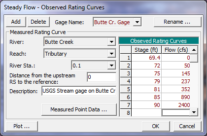
As shown in the figure above, the user can Add or Delete a rating curve by pressing one of the buttons at the top. For each rating curve the user is required to select the River, Reach, and River Station that corresponds to the location of the gage. If the gage is not located exactly at one of the user entered cross sections, select the cross section up stream of the gage and then enter a distance downstream from that section to the gage. A description can optionally be entered for the gage. Stage and flow values should be entered for the mean value rating curve at that gage location. In addition to the mean rating curve, the user can enter the actual measured points that went into developing the rating curve. This is accomplished by pressing the Measured Point Data button, which will pop up another editor. In the measured point data editor the user can enter the flow and stage for each measured point that has been surveyed for the gage. Additionally a description can be added for each point (i.e. 72 flood, slope-area measurement, etc…). If measured point data are also entered, then that data will show up on the rating curve plot when comparing the computed water surfaces to the observed.
Gate Openings. This option allows the user to control gate openings for any inline or lateral gated spillways that have been added to the geometric data. When this option is selected, a window will appear as shown in the figure below.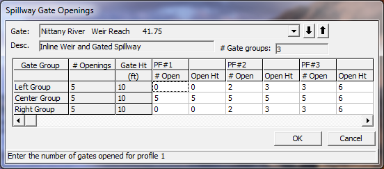
As shown in the figure above, for each profile the user can specify how many gates are opened per gate group, and at what elevation they are opened too. For the example shown in 6, there are three gate groups labeled "Left Group," "Center Group," and "Right Group." Each gate group has five identical gate openings. All of the gate openings have a maximum opening height of ten feet. For profile number 1, only the middle gate group is opened, with all five gates opened to a height of five feet. For the second profile, all three gate groups are opened. The Left gate group has two gates opened to three feet, the Center gate group has five gates opened to five feet, and the Right gate group has two gates opened for three feet. This type of information must be entered for all of the profiles being computed.
Optimize Gate Openings. This option allows the user to have the program compute a gate setting at a structure in order to obtain a user specified water surface upstream of the structure. Given a user entered flow and upstream stage for each profile, the program will iterate with different gate settings until the desired upstream water surface is obtained. This option is very handy when modeling dams and reservoirs.
Initial Split Flow Optimizations (LS and Pumps). This option allows the user to enter initial estimates of the flow that is leaving the main river through a lateral structure or a pump station. Flow values can be entered for each profile. When a value is entered for this option, that amount of flow is subtracted from the main river before the first profile is computed. This option can be useful in reducing the required computation time, or allowing the program to reach a solution that may not otherwise been obtainable.
Inline and Lateral Structure Outlet TS Flows: There is an option on the Inline Structure editor to add a time series of flows type of outlet. This is generally used for Unsteady flow modeling and representing hydropower flows. However, if you are running a model in Steady Flow mode, you can still use this feature. The flow data for this feature will be just the flow rate for this outlet for each profile. The flow entered is a portion of the total flow going through the inline structure for that specific profile.
Storage Area Elevations. This option allows the user to enter water surface elevations for storage areas that have been entered into the geometric data. Storage areas are most often used in unsteady flow modeling, but they may also be part of a steady flow model. When using storage areas within a steady flow analysis, the user is required to enter a water surface elevation for each storage area, for each profile.
Saving Steady Flow Data
The last step in developing the steady flow data is to save the information to a file. To save the data, select the Save Flow Data As from the File menu on the steady flow data editor. A pop up window will appear prompting you to enter a title for the data.
Importing Steady Flow Data from DSS
HEC-DSS is a data base system that was specifically designed to store data for applications in water resources. The HEC-DSS system can store almost any type of data, but it is most efficient at storing large blocks of data (e.g., time-series data). These blocks of data are stored as records in HEC-DSS, and each record is given a unique name called a "pathname." A pathname can be up to 391 characters long and, by convention, is separated into six parts. The parts are referenced by the letters A, B, C, D, E, and F, and are delimited by a slash "/" as follows: /A/B/C/D/E/F/
The pathname is used to describe the data in enough detail that various application programs can write to and read data from HEC-DSS by simply knowing the pathname. For more information about HEC-DSS, the user is referred to the "HEC-DSS, User's Guide and Utility Manuals" (HEC, 1995).
Many of the HEC application programs have the ability to read from and write to the HEC-DSS. This capability facilitates the use of observed data as well as passing information between software programs. The ability to read data from HEC-DSS has been added to HEC-RAS in order to extract flow and stage data for use in water surface profile calculations. It is a common practice to use a hydrologic model (i.e., HEC-HMS) to compute the runoff from a watershed and then use HEC-RAS to compute the resulting water surface profiles.
Reading data from HEC-DSS into HEC-RAS is a two-step process. First, the user must establish connections between HEC-RAS cross-section locations and pathnames contained in the HEC-DSS file. These connections are established by selecting the "Set Locations for DSS Connections" option from the File menu of the Steady Flow Data editor. When this option is selected, a window will appear as shown in the figure below. The user selects cross-section locations for DSS connections by selecting a River, Reach, and River Station, then pressing the "Add selected location to table" button. When this button is pressed, a new row will be added to the table at the top of the window. The user should do this for all the locations where they want to establish connections to HEC-DSS data.
The next step is to open a particular HEC-DSS file. The user has the option of either typing the filename in directly, or using the open button, which is right next to the filename field. Once a DSS file is selected, a listing of the pathnames for all of the data contained in that file will appear in the table at the bottom of the window. The user can establish connections to more than one DSS file if desired.
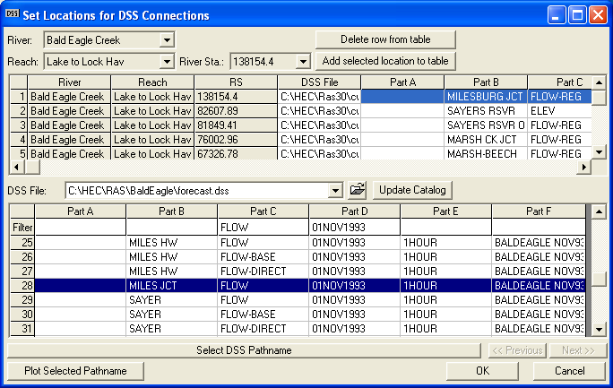
To establish the connection between an HEC-RAS cross section and a particular pathname in the DSS file, the user selects the row in the upper table that contains the river station that they want to connect data to. Next, they select the pathname that they want to connect to that river station from the lower table. Finally, they press the button labeled "Select DSS Pathname," and the pathname is added to the table at the top of the window.
To make it easier to find the desired pathnames, a set of pathname part filters were added to the top row of the lower table. These filters contain a list of all the DSS pathname parts contained within the currently opened DSS file. If the user selects a particular item within the list of one of the pathname parts, then only the pathnames that contain that particular pathname part will be displayed. These filters can be used in combination to further reduce the list of pathnames displayed in the table. When a particular filter is left blank, that means that pathname part is not being filtered.
Another feature on the editor to assist in selecting the appropriate pathnames is the "Plot Selected Pathname" button. This button allows the user to get a plot or a table of the data contained within any record in the DSS file. The user simply selects a DSS pathname, and then presses the Plot Selected Pathname button, and a new window will appear with a graphic of the data contained within that record.
Once all of the pathname connections are set, the user presses the OK button to close the editor. The next step is to import the data. This is accomplished by selecting "DSS Import" from the File menu of the Steady Flow Data editor. When this option is selected, a window will appear as shown in the figure below.
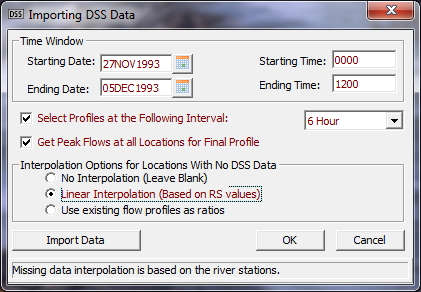
First the user sets a time window, which consists of a starting date and time and an ending date and time. When data are extracted from DSS, the program will only look at the data that is contained within the user specified time window.
Below the time window there are two options for selecting flow data to be extracted from the DSS file. The first option allows the user to pick off flow data at a specified time interval, starting with the beginning of the time window for the first profile. The second and subsequent profiles would be based on adding the user specified time interval to the start time of the time window. Flow data is extracted from the hydrographs at each of the locations being read from DSS. The second option listed on the window allows the user to get an overall peak flow for a profile computation. When this option is selected, the peak flow will be extracted from each hydrograph, within the time window specified. These peak flows will be made into the final profile in the flow data editor.
The bottom portion of the window contains options for interpolating flow data at locations that do not have hydrographs in the DSS file. After the flow data are read in, it will be necessary to interpolate flow data at all of the locations listed in the flow data editor that do not have values in the DSS file. Three options are available: no interpolation, linear interpolation, or using the flow data from an existing profile to calculated ratios for interpolating between points that have data. Once all the options are set, the user presses the "Import Data" button, to have the data imported and fill out the flow data editor.
Importing Steady Flow Data from an Existing Output Profile
This option allows the user to select an existing Plan from the current project, and to import flow data from that plans output into the current steady flow file. This can be a very handy option if you want to take the computed flows from an unsteady flow run and import them into a steady flow file, in order to make a steady flow analysis model. The user must already have all the flow change locations they want in the table first, before using this option.
Performing Steady Flow Calculations
Once all of the geometry and steady flow data have been entered, the user can begin calculating the steady flow water surface profiles. To perform the simulations, go to the HEC-RAS main window and select Steady Flow Analysis from the Run menu. The Steady Flow Analysis window will appear as in Figure 6 9 (except yours may not have a Plan title and short ID).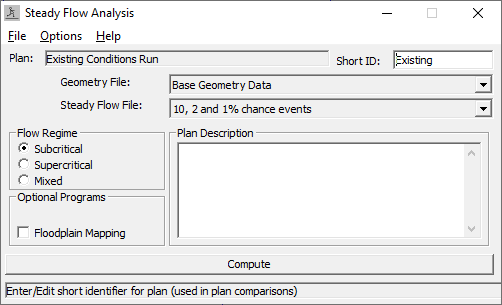
Simulation Options
The following is a list of the available simulation options under the Options menu of the Steady Flow Analysis window:
Encroachments. This option allows the user to perform a floodway encroachment analysis. For a detailed description of how to use the floodway encroachment capabilities of HEC-RAS, see Steady Flow Floodway Encroachment Analysis. For a description of how the encroachment calculations are performed for the various encroachment methods, see the Hydraulic Reference Manual.
Flow Distribution Locations. Flow Distribution Locations have been removed as a simulation option, and are now a geometry level option. Subdividing the left overbank, main channel, and right overbank, for the purpose of computing additional hydraulic information can now be done through the Htab Parameters menu in the Geometry Editor.
Conveyance Calculations. This option allows the user to tell the program how to calculate conveyance in the overbanks. Two options are available. The first option, At breaks in n values only, instructs the program to sum wetted perimeter and area between breaks in n values, and then to calculate conveyance at these locations. If n varies in the overbank the conveyance values are then summed to get the total overbank conveyance. The second option,
Between every coordinate point (HEC-2 style), calculates wetted perimeter, area, and conveyance between every coordinate point in the overbanks. The conveyance values are then summed to get the total left overbank and right overbank conveyance. These two methods can provide different answers for conveyance, and therefore different computed water surfaces. The At breaks in n values only method is the default.
Friction Slope Methods. This option allows the user to select one of five available friction slope equations, or to allow the program to select the method based on the flow regime and profile type. The five equations are:
- Average Conveyance (Default)
- Average Friction Slope
- Geometric Mean Friction Slope
- Harmonic Mean Friction Slope
- HEC-6 Slope Average Method
Set Calculation Tolerances. This option allows the user to override the default settings for the calculation tolerances. These tolerances are used in the solution of the energy equation. Warning !!! - Increasing the default calculation tolerances could result in computational errors in the water surface profile. The tolerances are as follows:
Water surface calculation tolerance: This tolerance is used to compare against the difference between the computed and assumed water surface elevations. When the difference is less than the tolerance, the program assumes that it has a valid numerical solution. The default value is 0.01.
Critical depth calculation tolerance: This tolerance is used during the critical depth solution algorithm. The default value is 0.01.
Maximum number of iterations: This variable defines the maximum number of iterations that the program will make when attempting to balance a water surface. The default value is 20.
Maximum difference tolerance: This tolerance is used during the balance of the energy equation. As the program attempts to balance the energy equation, the solution with the minimum error (assumed minus computed water surface) is saved. If the program goes to the maximum number of iterations without meeting the specified calculation tolerance, the minimum error solution is checked against the maximum difference tolerance. If the solution at minimum error is less than this value, then the program uses the minimum error solution as the answer, issues a warning statement, and then proceeds with the calculations. If the solution at minimum error is greater than the maximum difference tolerance, then the program issues a warning and defaults the solution to critical depth. The computations then proceed from there. The default value is 0.30.
Flow Tolerance Factor: This factor is only used in the bridge and culvert routines. The factor is used when the program is attempting to balance between weir flow and flow through the structure. The factor is multiplied by the total flow. The resultant is then used as a flow tolerance for the balance of weir flow and flow through the structure. The default value is 0.001
Maximum Iteration in Split Flow: This variable defines the maximum number of iterations that the program will use during the split flow optimization calculations. The default value is 30.
Flow Tolerance Factor in Weir Split Flow: This tolerance is used when running a split flow optimization with a lateral weir/gated spillway. The split flow optimization continues to run until the guess of the lateral flow and the computed value are within a percentage of the total flow. The default value for this is 2 percent (.02).
Maximum Difference in Junction Split Flow: This tolerance is used during a split flow optimization at a stream junction. The program continues to attempt to balance flow splitting from one reach into two until the energy gradelines of the receiving streams are within the specified tolerance. The default value is 0.02.
Each of these variables has an allowable range and a default value. The user is not allowed to enter a value outside of the allowable range.
Critical Depth Output Option. This option allows the user to instruct the computational program to calculate critical depth at all locations.
Critical Depth Computation Method. This option allows the user to select between two methods for calculating critical depth. The default method is the Parabolic Method. This method utilizes a parabolic searching technique to find the minimum specific energy. This method is very fast, but it is only capable of finding a single minimum on the energy curve. A second method, Multiple Critical Depth Search, is capable of finding up to three minimums on the energy curve. If more than one minimum is found the program selects the answer with the lowest energy. Very often the program will find minimum energies at levee breaks and breaks due to ineffective flow settings. When this occurs, the program will not select these answers as valid critical depth solutions, unless there is no other answer available. The Multiple Critical Depth Search routine takes a lot of computation time. Since critical depth is calculated often, using this method will slow down the computations. This method should only be used when you feel the program is finding an incorrect answer for critical depth.
Flow Optimizations. This option allows the user to have the program optimize the split of flow at lateral structures, lateral diversions, stream junctions, and pump stations. When this option is selected, a window will appear as shown in the figure below. There are four tabs to choose from. One tab is for each of the following: Junctions; Lateral Weirs/Diversions; Reach-Storage Areas; and Pump Stations.
When the Lateral Weir/Diversion tab is selected, a table with all of the lateral weirs/spillways and rating curves defined in the model will be displayed. To have the program optimize the split of flow between the main stream and a lateral weir/spillway (or rating curve), the user simply checks the column labeled "Optimize." If you do not want a particular lateral weir/spillway to be optimized, the user should not check the box. For the first iteration of the flow split optimization, the program assumes that zero flow is going out of the lateral structure. Once a profile is computed, the program will then compute flow over the lateral structure. The program then iteratively reduces the flow in the main channel, until a balance is reached between the main river and the lateral structure. The user has the option to enter an initial estimate of the flow going out the lateral structure. This can speed up the computations, and may allow the program to get to a solution that may not have otherwise been possible. This option is available by selecting "Initial Split Flow Values" from the "Options" menu of the Steady Flow Data editor.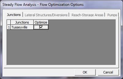
When the Junction tab is selected, the table will show all of the junctions in the model that have flow splits. To have the program optimize the split of flow at a junction, check the optimize column, otherwise leave it unchecked. Flow optimizations at junctions are performed by computing the water surface profiles for all of the reaches, then comparing the computed energy grade lines for the cross sections just downstream of the junction. If the energy in all the reaches below a junction is not within a specified tolerance (0.02 feet), then the flow going to each reach is redistributed and the profiles are recalculated. This methodology continues until a balance is reached.
When the Reach – Storage Areas tab is selected, a window will appear displaying all of the storage areas that are upstream boundaries to river reaches. If optimization is set to on for a particular storage area, the program will optimize the amount of flow coming out of the storage area, based on the user specified elevation of the storage area.
The final tab is for Pumps. When this tab is pressed a table will appear showing all of the locations where pump stations are connected to the main rivers. The user can then turn on optimization for the split of flow between the main river and the pump station.
Check Data Before Execution. This option provides for comprehensive data input checking. When this option is turned on, data input checking will be performed when the user presses the compute button. If all of the data are complete, then the program allows the steady flow computations to proceed. If the data are not complete, or some other problem is detected, the program will not perform the steady flow analysis, and a list of all the problems in the data will be displayed on the screen. If this option is turned off, data checking is not performed before the steady flow execution. The default is that the data checking is turned on.
Set Log File Output Level. This option allows the user to set the level of the Log file. The Log file is a file that is created by the computational program. This file contains information tracing the program process. Log levels can range between 0 and 10, with 0 resulting in no Log output and 10 resulting in the maximum Log output. In general, the Log file output level should not be set unless the user gets an error during the computations. If an error occurs in the computations, set the log file level to an appropriate value. Re-run the computations and then review the log output, try to determine why the program got an error.
When the user selects Set Log File Output Level, a window will appear as shown in Figure 6-12. The user can set a "Global Log Level," which will be used for all cross sections and every profile. The user can also set log levels at specific locations for specific profiles. In general, it is better to only set the log level at the locations where problems are occurring in the computations. To set the specific location log level, first select the desired reach and river station. Next select the log level and the profile number (the log level can be turned on for all profiles). Once you have everything set, press the Set button and the log level will show up in the window below. Log levels can be set at several locations individually. Once all of the Log Levels are set, press the OK button to close the window.
View Log File. This option allows the user to view the contents of the log file. The interface uses the Windows Write program to accomplish this. It is up to the user to set an appropriate font in the Write program. If the user sets a font that uses proportional spacing, the information in the log file will not line up correctly. Some fonts that work well are: Line Printer; Courier (8 pt.); and Helvetica (8 pt.). Consult your Windows user's manual for information on how to use the Write program.
View Runtime Messages File. This option will allow the user to open a file that contains the runtime messages from the last time the Steady Flow model was computed.