Land Classification Layers

The use of spatially varied data across the model domain is characterized in RAS Mapper through the creation of land classification layers. Land Classification layers can be used to for identifying specific parameter values for Manning's n values, soils data, and infiltration parameters. The basic process of using data based on land classification is to import either gridded data or polygon shapefiles that have a unique value upon which they can be classified. Once the data are used to create a RAS Layer, you can define individual parameters for each unique land classification layer.

The Land Classification layers currently supported in RAS Mapper are referred to as a Land Cover layer, Percent Impervious Layer, Soils Layer, Infiltration layer, or Sediment Bed Materials Layer. Land Classification layers have a sub-layer associated with it named "Classification Polygons". Classification Polygons are used to define a land classification or to override an area in the Land Classification layer.

Classification names cannot have special characters in the name ( specifically, "/" and "\", which are found in the NLCD data). A red asterisk will inform you the dataset is invalid.

Version 6.0 incorrectly allowed this. If your dataset has invalid classification names, you can right-click on the land cover layer to fix the names using the Sanitize Classification Names menu item.

New Layers

New layers are created by selecting the he Map Layers | Create New RAS Layer menu and selecting the layer type of interest. This will invoke a layer import dialog. If you wish to create an empty layer to digitize spatial information, you do so by pressing the Create Empty layer button before adding any data (as shown in the figure below).

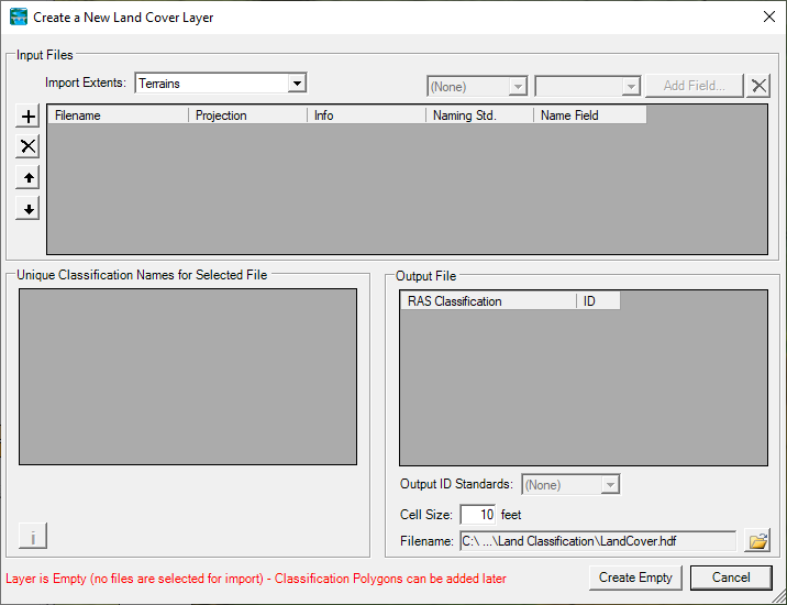
To create an EMPTY Classification Layer, press the Create Empty button without adding any files. An empty Classification Layer can then be used to add Classification Polygons. This is true for Land Cover, Soils, and Infiltration Layers.

Land Cover Layer

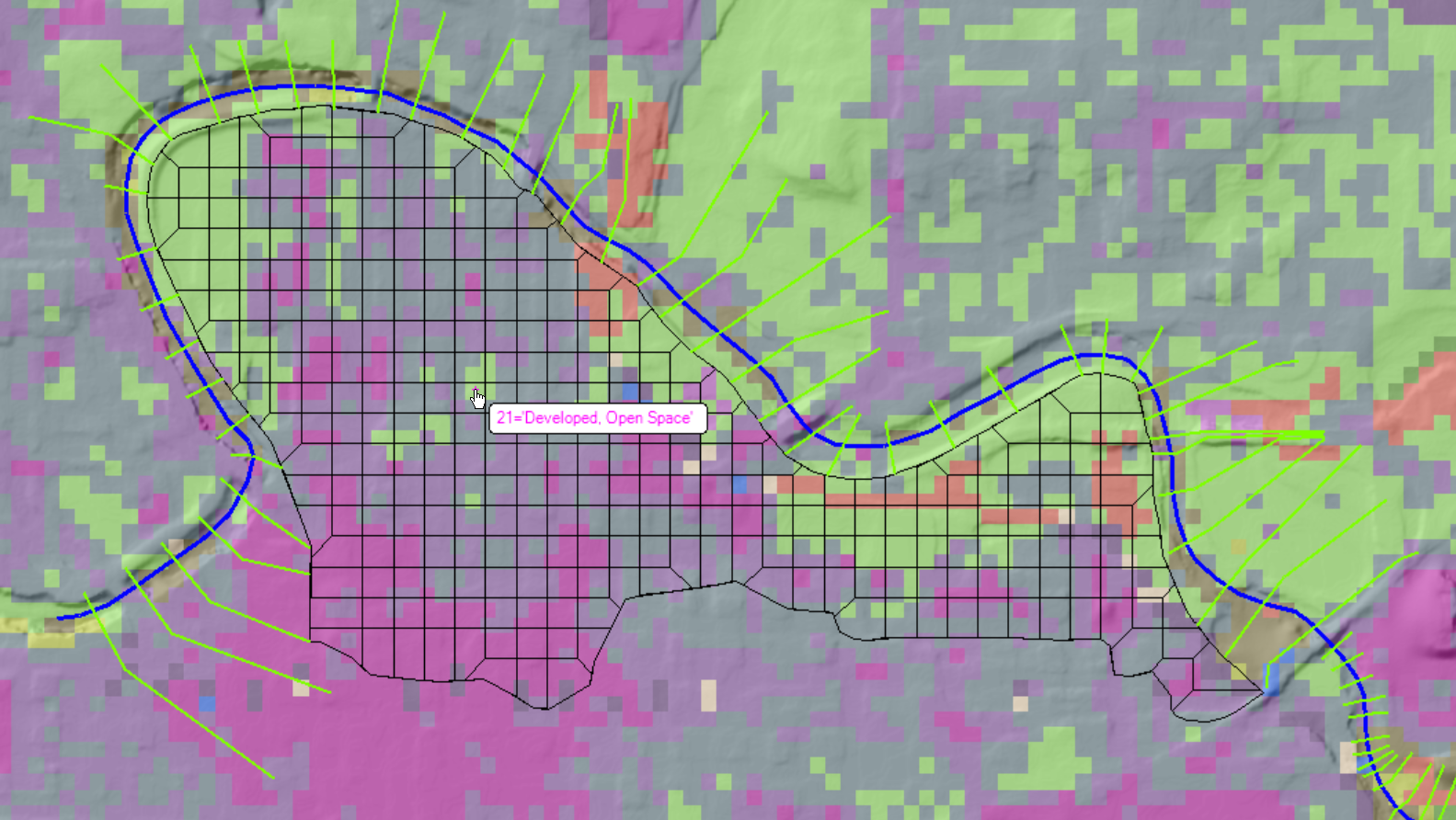
Support for the use of Land Cover data for estimating the spatial distribution of surface roughness and defining the percent impervious area in HEC-RAS is available in RAS Mapper. There are several published data sources for Land Cover data in both gridded and polygon format; however, the most prominent data sources are those provided by the National Land Cover Database (https://www.mrlc.gov/) and the USGS (USGS vector data: https://water.usgs.gov/GIS/dsdl/ds240/index.html). These small-scale datasets typically are not sufficient for defining surface roughness for hydraulic modeling; however, they show general trends in land cover across broad areas. Channel data will NOT be sufficient for estimation of roughness coefficients requiring the user to supplement the data with information from aerial photographs in field data.

The Land Cover layer is used in HEC-RAS as a surrogate for roughness coefficients. RAS Mapper supports the use of multiple grids or polygon shapefiles having a unique name field to classify the land. During the creation of the Land Cover layer, the layers then prioritized (the highest priority layer above lower priority layers) and are converted to a single integer raster (default filename is “LandCover.tif”) using a specified cell size (default cell size value is 10). The Land Cover GeoTiff values are mapped through a unique description/name (typically from the Land Cover) to a Manning’s n value and/or percent impervious area. The Land Cover dataset can then be used to extract spatially distributed n values for Cross Sections and 2D Flow Area meshes and impervious area for 2D Flow Areas.

Creating the Land Cover Layer

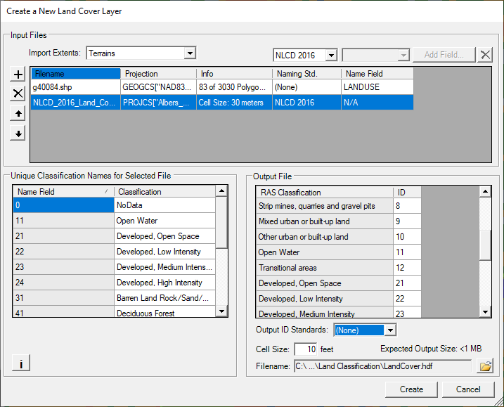
A new Land Cover Layer is created by selecting one or many raster or polygon shapefile datasets and importing them into a single layer. This is done selecting the Map Layers | Create New RAS Layer | Land Cover Layer to invoke the New Land Cover Layer dialog, shown in the figure below. A series of tables are provided to allow the user to define a unique classification name. Once a description has been provided, a “LandCover” grid ("LandCover.hdf" and "LandCover.tif") will be created, using the specified Cell Size.

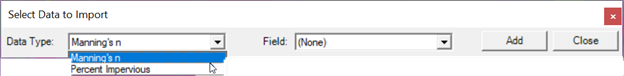
New Land Cover layer creation dialog.

If you are importing a shapefile that already has data defined for the Manning's n values or percent impervious, you can use the "Add Field" button to include those data fields and map the data to the RAS Mapper data type.

Import Extents are used to limit the amount of data that RAS will process. The default value of “Terrains” means that only data within the bounds of the RAS Terrains will be evaluated and converted to the LandCover grid. Additional options include: “Geometries”, “Terrains and Geometries”, “Current View”, and “Entire Input File(s)”. The Import Extents should be established prior to adding Input Files.

Input Files are added to the dialog through the Add Files button. These are the files that will be imported and evaluated by the priority as defined in the list. The land cover file at the top of the list has the highest priority when evaluating the Land Cover Layer.

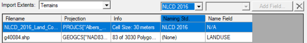
Raster data is treated differently from polygon shapefile datasets. Raster data will be identified through integer values. Therefore, the user will have to establish a naming standard. Three default naming standards are available for raster datasets to link the integer values to a common description based on the NLCD 2016 naming standard, the Anderson Level II naming standard (USGS data), and the NOAA C-CAP system.

Naming Standard – The “Naming Std.” field is provided to help the user auto-populate the RAS Identifier. If the data uses “NLCD2016” or the “USGS Anderson Level II” naming standards, the predefined names will be populated based on the integer values of the dataset. (In the figure above, “Anderson II” has been selected for the Naming Standard.)

If using polygon datasets, the user will also have the ability to specify the unique “Name Field” which selects the field that has a unique name/description that classifies the land cover polygon.

Name Field (shapefile only) – The “Name Field” is used to select the Shapefile field that holds the descriptions for the land cover data and will automatically use those names for the RAS Identifier. (In the figure below, “LANDUSE” has been selected for the Name Field.)

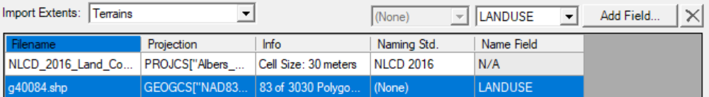
The polygon dataset may also have associated data that can be imported along with the classification name. The Add Field button can be used to import the data field and have it mapped as either Manning's n values or Percent Impervious.

Add Field (Shapefile only) – The “Add Field” is provided to allow the user to select the Shapefile field that contains Manning’s n Value or Percent Impervious information.

Selected File Land Cover Identifiers are defined per dataset. Data is displayed for whichever Input File is selected. The user can then enter the RAS Identifier (e.g. name or description) to associate with raster/shapefile polygon value.

Output File information specifies what will be in the Land Cover layer that is created by RAS. A Land Cover raster layer will be created based on the defined ID values (with the 0 value is reserved for No Data values) and will be linked to the unique names. The Output File information is a summary of all Input File values and user-specified data.

Cell Size indicates the grid cell size of the raster dataset that will be created to associated land cover.

Filename is the user-defined name of the Land Cover dataset (the default name is "LandCover"). The LandCover.hdf file will be created along with the LandCover.tif raster dataset. The LandCover.hdf file will also contain lookups between the raster cell ID and the unique name. The Land Cover dataset will be created by default in the RAS Land Classification t folder in the project projection.

When created, the Land Cover layer will be automatically added to the display.

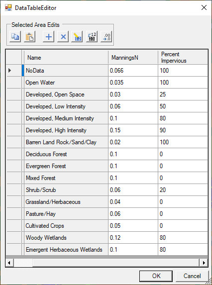
Parameterizing Land Cover Data

At this point, the data has been classified. To parameterize the data, right-click on the land cover layer and select the Edit Land Cover Data menu item. Land Cover layers will provide the possibility to paramaterize Manning's n value and Percent Impervious data. Once the data have been entered, press the OK button to save the changes.

Soils Layer

Soils data is used to help define the parameters used in for the selected Infiltration Method. Soils data information can be quite complex. Vector (shapefile) data from the SSURGO database can be downloaded from the NRCS (https://websoilsurvey.sc.egov.usda.gov/App/WebSoilSurvey.aspx). The data comes as a shapefile with an abbreviated soils name and unique key. Numerous tables are also included, however, to use the tabular data, you will need to have an understanding of the tables (metadata and table columns information can be accessed here: https://www.nrcs.usda.gov/wps/portal/nrcs/detail/soils/survey/geo/?cid=nrcs142p2_05363) and join the data from the tables using other software like a GIS. Data are also available in a geodatabase format from the gSSURGO database (https://datagateway.nrcs.usda.gov/GDGOrder.aspx). RAS Mapper has the capability to import the gSSURGO data.

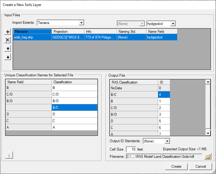
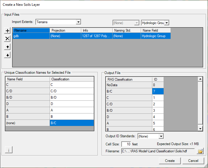
Creating a Soils Layer is similar to the Land Cover Layer. Select the Map Layers | Create New RAS Layer | Soils Layer to invoke the Create New Soils Layer dialog. If you are adding soils in shapefile format, select the field name that provides a unique name convention for the soils layer, such as "Hydrologic Group" or "Texture Class". Adding soils data from a standard coordinate system will take a moment to load the data as all of the polygons must be reprojected to the coordinate system used for the project. If using the gSSURGO geodatabase (discussed below), other field choices will be provided for you.

Pressing the Create button will create a “Soils” grid ("Soils.hdf" and "Soils.tif") will be created, using the specified Cell Size.

Importing gSSURGO Data

If you adding gSSURGO data, you will need to select the "GSSURGO" name from the file type list. Navigate to the file geodatabase (which is a folder). Pick a file inside of the database ("gdb" is a good choice), choose the Open button. RAS Mapper willl recognize and interpret the database, preparing it for import.

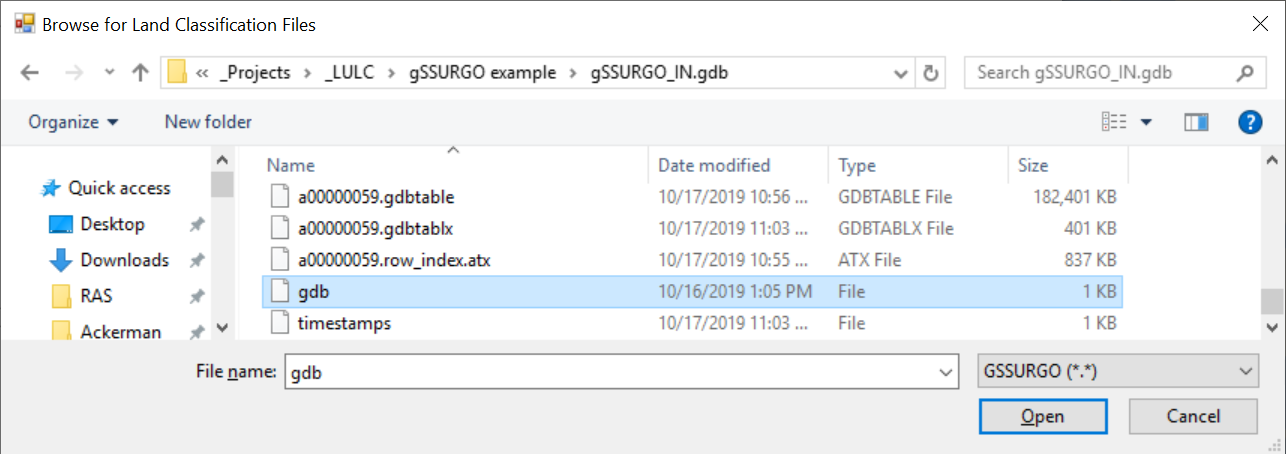
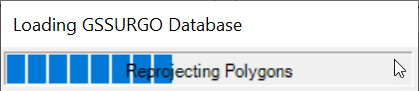
The data will then be imported, converted from the geodatabase to raster and projected to the RAS Mapper coordinate system. As the data are loaded, the user will be informed with a progress bar.

By default, RAS Mapper will choose to bring the data in classified on the "Hydrologic Group" field. Other options include the "Texture Group", "Map Unit Key", "Map Unit Symbol", or a the combination of hydrologic group and texture group "Merged Hydr : Texture". Select the Name Field to classify the data. It is likely that some of the SSURGO data will not be classified; in this case, RAS Mapper will classify those areas with the "none" keyword. It is the user's responsibility to provide a classification for that data.

Verify the output file Cell Size and Filename. Press Create to create the soils layer.

Infiltration Layer

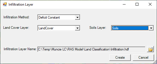
RAS Mapper allows for the creation of an Infiltration Layer. An Infiltration Layer defines the Infiltration Method (Deficit Constant, SCS Curve Number, or Green and Ampt) that will be used for surface losses from a precipitation event. There are two different ways to generate an Infiltration Layer in RAS Mapper to represent infiltration parameters: (1) using and existing RAS Land Cover layer or RAS Soils layer or the intersection of a Land Cover layer and Soils layer or (2) to use a single classification shapefile layer to define the infiltration parameters. The approach used to create an infiltration layer for parameterization will depend on the selected infiltration method and data available.

Using a Land Cover and Soils Layer

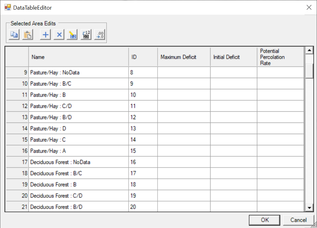
This will create a complex table which cross reference the Land Cover and Soils classifications from which you can parameterize the infiltration data. To create a complex Infiltration layer, select Map Layers | Create New RAS Layer | Infiltration Layer from Land Cover / Soils Layers menu item. A dialog will be provided to allow the user to select the Infiltration Method, Land Cover Layer, and Soils Layer and provide the new Infiltration Layer name. Note, that you do not need to specify both a Land Cover layer and a Soils Layer.

Press the Create button to create a new raster layer that is the intersection of the land cover and soils layers. As shown in the figure below, the intersection of the layers can become quite complex, creating a table with rows for each overlapping classification from the base layers. Depending on the infiltration method selection, additional columns for the required parameters will be provided.

Using a Classification Shapefile Layer

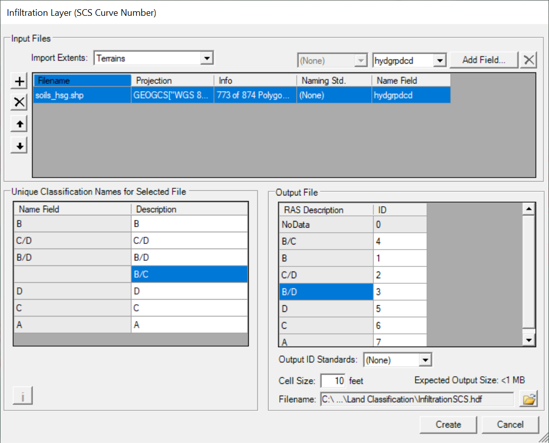
To use a single classification layer, select Map Layers | Create New RAS Layer | Infiltration Layer from Shapefile | Method menu item. The Create New Infiltration Layer dialog will come up allowing you to choose the shapefile of interest. Once the shapefile has been selected, select the unique classification name (like "Hydrologic Soils Group") to import the data, as shown in the figure below.

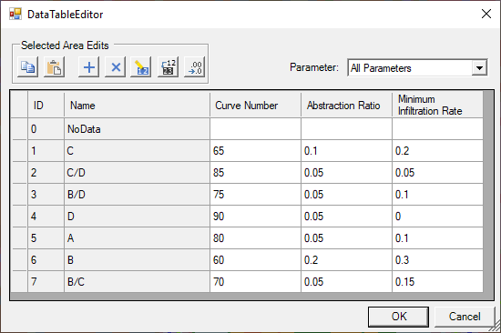
Once the data has been imported, you will need to enter infiltration parameters by right-clicking on the Infiltration Layer and selecting Edit Infiltration Data. A table will be provided with the infiltration parameter based on the Infiltration Method (Deficit Constant, SCS Curve Number, or Green and Ampt) selected.

Classification Polygons

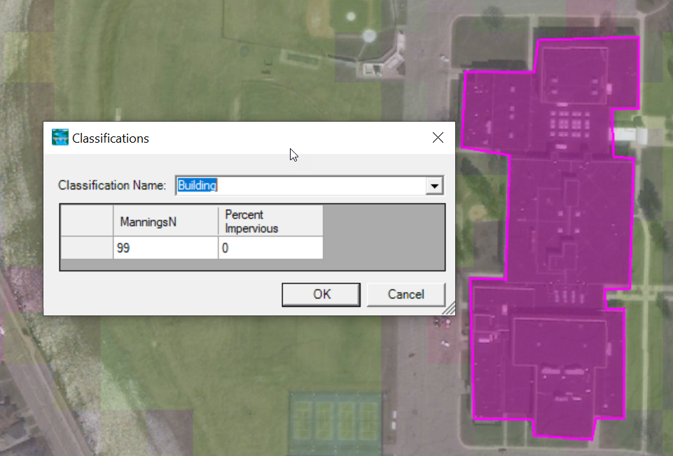
Land Classification layers have a sub-layer associated with it named "Classification Polygons". These are used to further define a land classification or to override an area in the Land Classification layer. Use this layer with the Editing tools to create polygons. Once a polygon has been created, an editor will be provided allowing the user to select the classification or to specify a new unique Classification Name and provide the associated parameter values. Note: if you type in a parameter for an existing classification, it will replace the existing data for the that class.

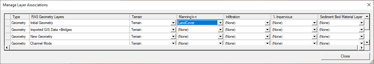
Associating the Land Classification Layer with a Geometry

Once you have develop classification layers and entered parameter values, you will need to associate the layers with the geometry. Depending on the type of study and data prepared, you may only have to associate the Land Cover layer with the Manning's n value data (and Terrain layer).

NLCD - Manning's n Values Reference Table¹

NLCD Value	n Value Range	Description
11	0.025 - 0.05	Open Water- areas of open water, generally with less than 25% cover of vegetation or soil.
12	n/a	Perennial Ice/Snow- areas characterized by a perennial cover of ice and/or snow, generally greater than 25% of total cover.
21	0.03 - 0.05	Developed, Open Space- areas with a mixture of some constructed materials, but mostly vegetation in the form of lawn grasses. Impervious surfaces account for less than 20% of total cover. These areas most commonly include large-lot single-family housing units, parks, golf courses, and vegetation planted in developed settings for recreation, erosion control, or aesthetic purposes.
22	0.06 - 0.12	Developed, Low Intensity- areas with a mixture of constructed materials and vegetation. Impervious surfaces account for 20% to 49% percent of total cover. These areas most commonly include single-family housing units.
23	0.08 - 0.16	Developed, Medium Intensity -areas with a mixture of constructed materials and vegetation. Impervious surfaces account for 50% to 79% of the total cover. These areas most commonly include single-family housing units.
24	0.12 - 0.20	Developed High Intensity-highly developed areas where people reside or work in high numbers. Examples include apartment complexes, row houses and commercial/industrial. Impervious surfaces account for 80% to 100% of the total cover.
31	0.023 - 0.030	Barren Land (Rock/Sand/Clay) - areas of bedrock, desert pavement, scarps, talus, slides, volcanic material, glacial debris, sand dunes, strip mines, gravel pits and other accumulations of earthen material. Generally, vegetation accounts for less than 15% of total cover.
41	0.10 - 0.20	Deciduous Forest- areas dominated by trees generally greater than 5 meters tall, and greater than 20% of total vegetation cover. More than 75% of the tree species shed foliage simultaneously in response to seasonal change.
42	0.08 - 0.16	Evergreen Forest- areas dominated by trees generally greater than 5 meters tall, and greater than 20% of total vegetation cover. More than 75% of the tree species maintain their leaves all year. Canopy is never without green foliage.
43	0.08 - 0.20	Mixed Forest- areas dominated by trees generally greater than 5 meters tall, and greater than 20% of total vegetation cover. Neither deciduous nor evergreen species are greater than 75% of total tree cover.
51	0.025 - 0.05	Dwarf Scrub- Alaska only areas dominated by shrubs less than 20 centimeters tall with shrub canopy typically greater than 20% of total vegetation. This type is often co-associated with grasses, sedges, herbs, and non-vascular vegetation.
52	0.07 - 0.16	Shrub/Scrub- areas dominated by shrubs; less than 5 meters tall with shrub canopy typically greater than 20% of total vegetation. This class includes true shrubs, young trees in an early successional stage or trees stunted from environmental conditions.
71	0.025 - 0.05	Grassland/Herbaceous- areas dominated by gramanoid or herbaceous vegetation, generally greater than 80% of total vegetation. These areas are not subject to intensive management such as tilling, but can be utilized for grazing.
72	0.025 - 0.05	Sedge/Herbaceous- Alaska only areas dominated by sedges and forbs, generally greater than 80% of total vegetation. This type can occur with significant other grasses or other grass like plants, and includes sedge tundra, and sedge tussock tundra.
73	n/a	Lichens- Alaska only areas dominated by fruticose or foliose lichens generally greater than 80% of total vegetation.
74	n/a	Moss- Alaska only areas dominated by mosses, generally greater than 80% of total vegetation.
81	0.025 - 0.05	Pasture/Hay-areas of grasses, legumes, or grass-legume mixtures planted for livestock grazing or the production of seed or hay crops, typically on a perennial cycle. Pasture/hay vegetation accounts for greater than 20% of total vegetation.
82	0.020 - 0.05	Cultivated Crops -areas used for the production of annual crops, such as corn, soybeans, vegetables, tobacco, and cotton, and also perennial woody crops such as orchards and vineyards. Crop vegetation accounts for greater than 20% of total vegetation. This class also includes all land being actively tilled.
90	0.045 - 0.15	Woody Wetlands- areas where forest or shrubland vegetation accounts for greater than 20% of vegetative cover and the soil or substrate is periodically saturated with or covered with water.
95	0.05 - 0.085	Emergent Herbaceous Wetlands- Areas where perennial herbaceous vegetation accounts for greater than 80% of vegetative cover and the soil or substrate is periodically saturated with or covered with water.

¹Manning's n values adapted from Chow (1959), excluding "Developed" land type. These n values are for appreciable depths of flow and are not meant for shallow overland flow. Shallow, overland flow Manning's n values are generally much higher, due to the relative roughness compared to the flow depth.

Using Land Cover for Manning's n Values

Once you have a Land Cover layer created in RAS Mapper, you can used it to associate Manning's n values. This is discussed in the Geometry Data | Manning's n Values section .