Download PDF
Download page Mapping Options.
Mapping Options
Render Mode
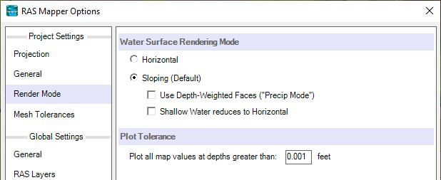
For 2D models, water surfaces within the cell are interpolated between computation points and face points. How the interpolation is performed, however, is slightly different based on the Render Mode when evaluating the water surface. The Render Modes available within RAS Mapper are characterized as either Sloping or Horizontal. These Render Modes are available from the Options | Render Mode menu item or by clicking the  Render Mode button. The mapping options are shown in the figure below. The Sloping method is the default method.
Horizontal Water Surface
The Horizontal water surface rendering mode plots the computed water surface as horizontal in each 2D Area cell. This option fills each 2D cell to the water surface as computed in the 2D simulation. In areas where the terrain has significant relief between 2D cells this plotting option can produce a “patchwork” of isolated inundated areas when visualizing flood depths. These isolated inundation areas are more visible in areas of steep terrain, using large grids cells, with shallow flood depths. This method is a volume conservative approach and should be used to generate stored maps where water volume will be used for further calculations.
Sloping Water Surface
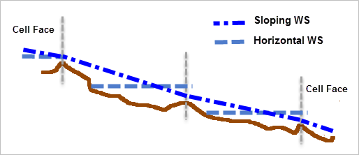
The Sloping water surface rendering mode plots the computed water surface by interpolating water surface elevations from each 2D cell face. This option of connecting each cell face provides a visualization for a more continuous inundation map. The more continuous inundation map, looks more realistic; however, under some circumstances it can also have the appearance of more water volume in the 2D cells than what was computed in the simulation. This problem generally occurs in very steep terrain with large 2D grid cells. This sloping water surface approach is most helpful when displaying shallow inundation depths in areas of steep terrain. This method is not a volume conservative approach. Water most likely will "be created" during the interpolation. This is the default rendering mode.
- Depth-weighted: weighting water surface elevations by face depths so that deep faces have more effect than shallow faces. This plot option is helpful to understand situations in steep terrain where shallow flow transitions to deeper flow (such as rain on grid situations).
- Shallow water reduces to horizontal: if RAS computes flow to be shallow for a particular 2D cell, inundation will be plotted with a horizontal water surface. This plot option will show more water than the default render mode and attempts to render some water where cells would typically be dry with the normal Sloping method.
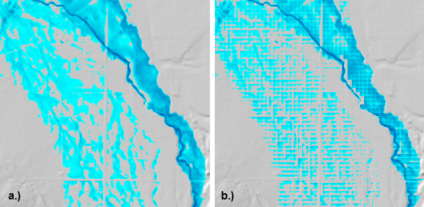
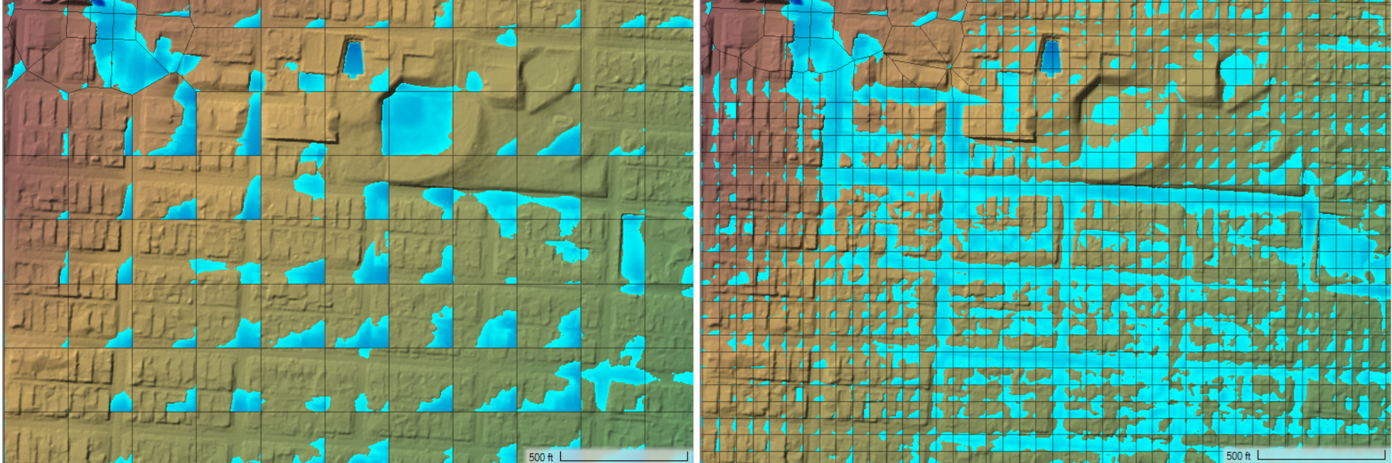
The impacts of the two different render modes (a) sloping and (b) horizontal are shown based on inundation depth in the figure below.
The Plot all map values with a depth greater than option allows for cleaner mapping within specified calculation tolerances.
A comparison of inundation mapping results using the Sloping method (with depth-weighting and horizontal for shallow water options) for two different grid cell sizes is shown below. HEC-RAS is able to properly route flow using the subgrid bathymetry, but RAS Mapper needs smaller cells to improve mapping. With the larger grid cells, the interpolation surface does not know how to distribute flow with each cell.
Additional Plot Options
Along with the general mapping capabilities, there are additional plot options available to assist you in the analysis of simulation results. These plot options are available from the Layer Properties for each of the RAS Results Map layers.
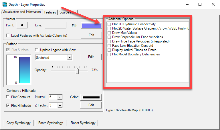
Plot 2D Hydraulic Connectivity
This plot option allows you to identify how water is connected from cell to cell. To create this "flow network", adjacent cells are connected by a blue line if the computed water surface elevation is higher than the minimum ground surface elevation of their shared face. The Hydraulic Connectivity plot is a good way to identify high ground in the terrain and identify areas in the 2D mesh that should be refined.
Examples of the hydraulic connectivity are shown below. Isolated pockets of water and high-ground locations become apparent when using this option.
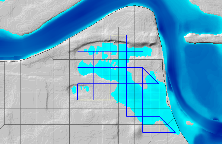
Isolated pockets of water indicate that smaller cell sizes or breaklines may be necessary.
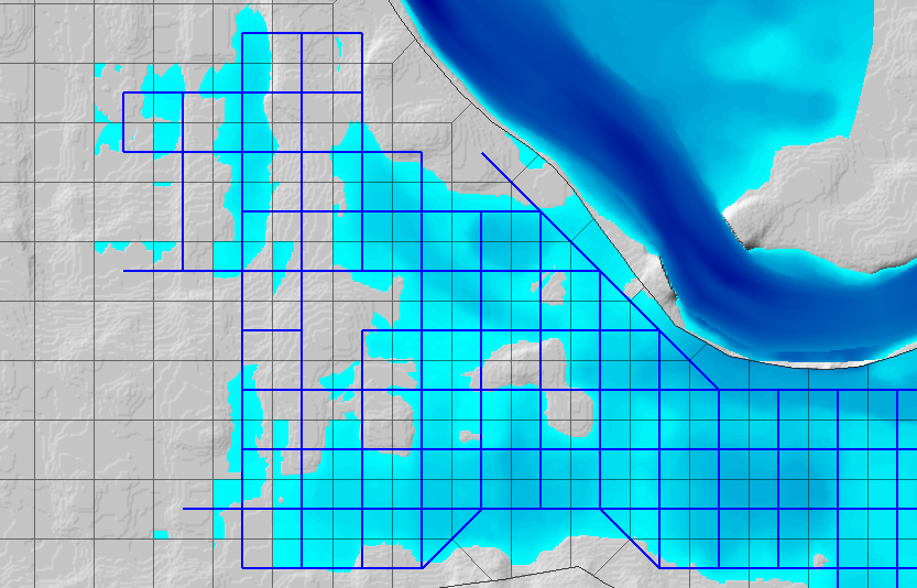
Disconnected flow and flow splits become apparent when using the hydraulic connectivity plot. Use breaklines to refine the 2D mesh.
Plot 2D Water Surface Gradient
This plot option allows you to identify how water is connected from cell to cell. To create this "flow network", the computed water surface for each cell is connected by a color-coded arrow to indicated the most-likely direction of flow and the "type" of flow. The arrow color and general description of the flow is summarized in the table below.
| Color | General Flow Description |
|---|---|
Blue | Normal flow. Flow where the upstream water surface elevation is greater than the downstream water surface elevation and flow is with the predominant velocity. Interpolation of water surface elevations is appropriate. |
Yellow | Shallow depth of flow. Water is moving from high ground to low ground but flow is not of significant depth over the cell face; however, it is expected to be hydraulically connected. Interpolation of water surface elevations would not appropriate for spreading the water out. |
Green | Intermediate depth of flow. While not deep, flow is expected over the adjacent cell face. |
Gray | Backwater. In this case the downstream (based on velocity) water surface elevation is greater than the upstream water surface elevation. Typically, the terrain and the water surface slope have adverse slopes: the cell with the higher water surface elevation has lower terrain elevation. |
Pink | Critical. Flow most likely passes through critical depth over a cell face. This is determined by looking at the water surface elevations adjacent to a face and comparing them to the minimum face elevation. |
It should be noted that the hydraulic connectivity is based solely on the property tables for each 2D Cell Face. If the hydraulic computations were modified by a 2D Connection, it will not be reflected in the flow network model (so it might look like flow is over-topping a levee at the wrong location). An example is shown below with flow network for a model with a levee. The water surface gradient arrows (left figure) improperly show water flowing over the top of the levee. Water was able to leak behind the levee and the algorithm used to connect cells is simply looking at differences in water surface elevations.
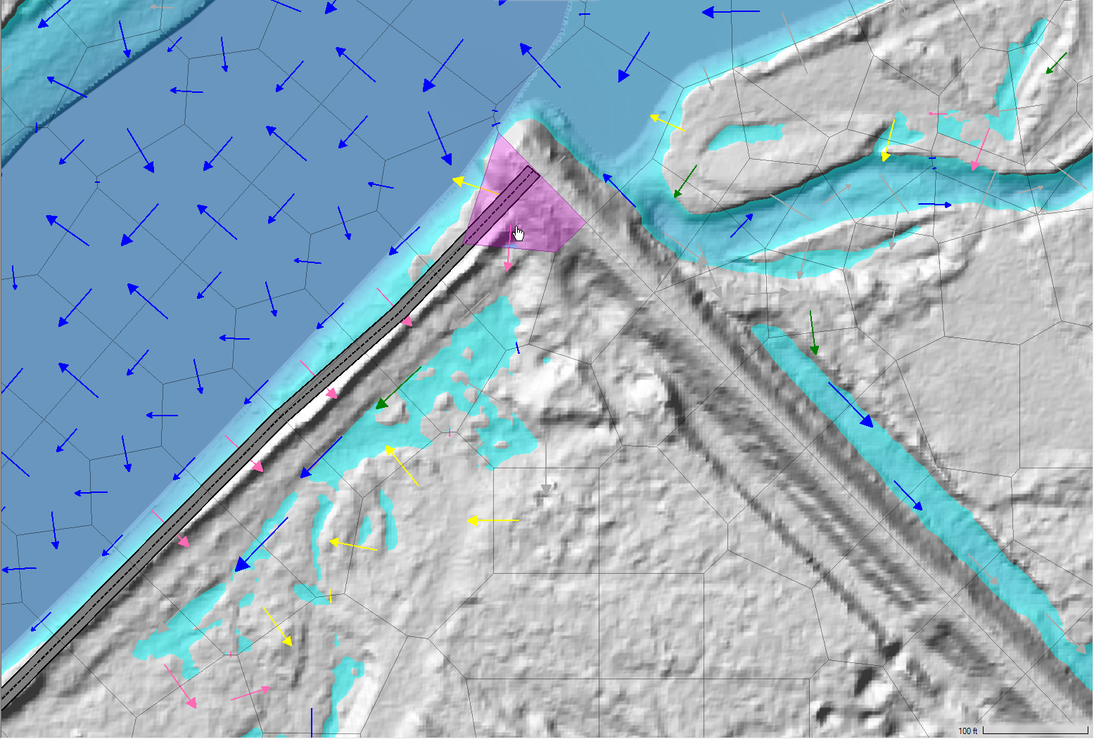
Improper mesh development is allowing water to leak around high ground behind the levee (highlighted cell). Water is not flowing over the levee as indicated by the velocity arrows.
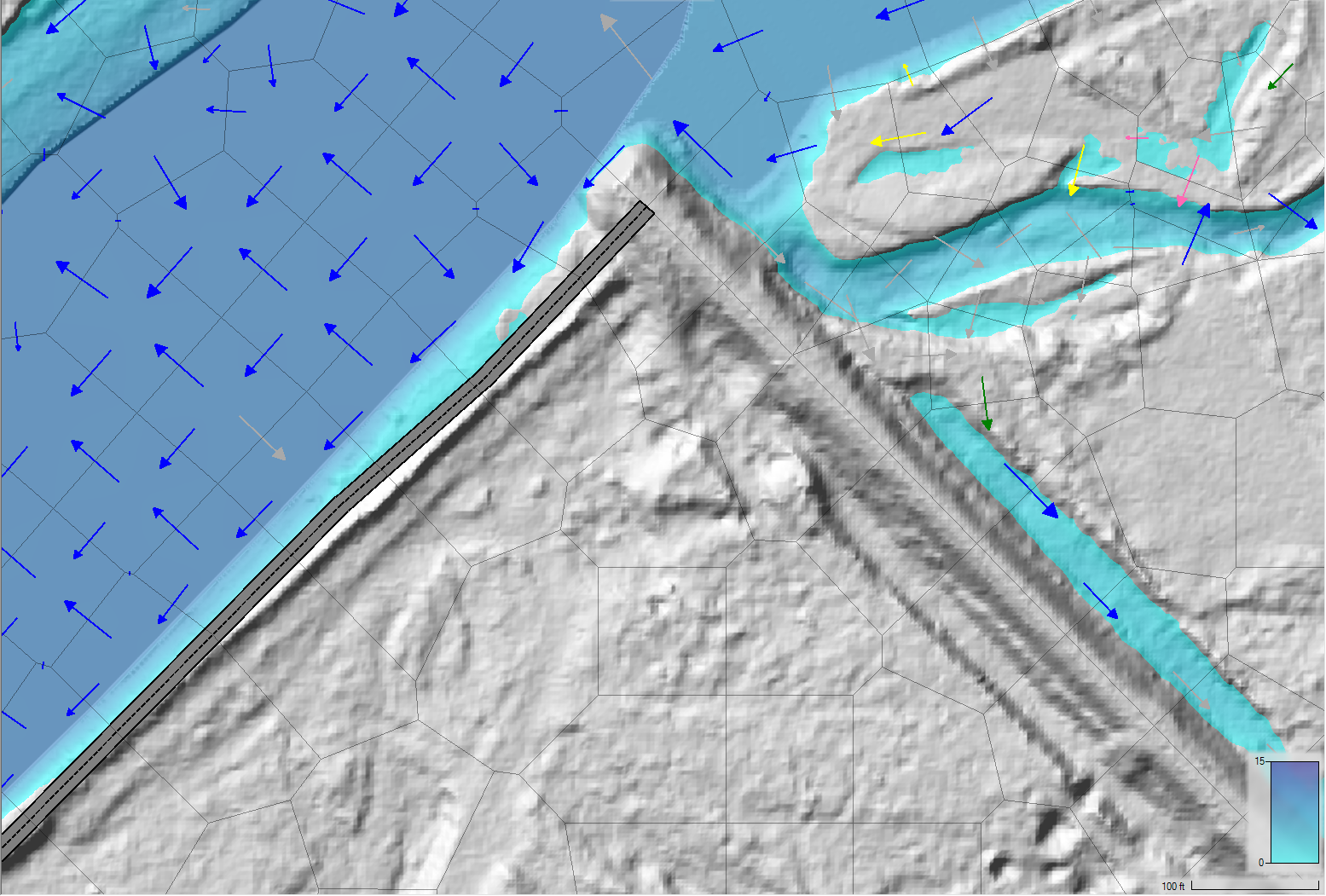
Properly enforced hydraulic structure. Flow is computed, as expected, and doesn't pass behind the levee.
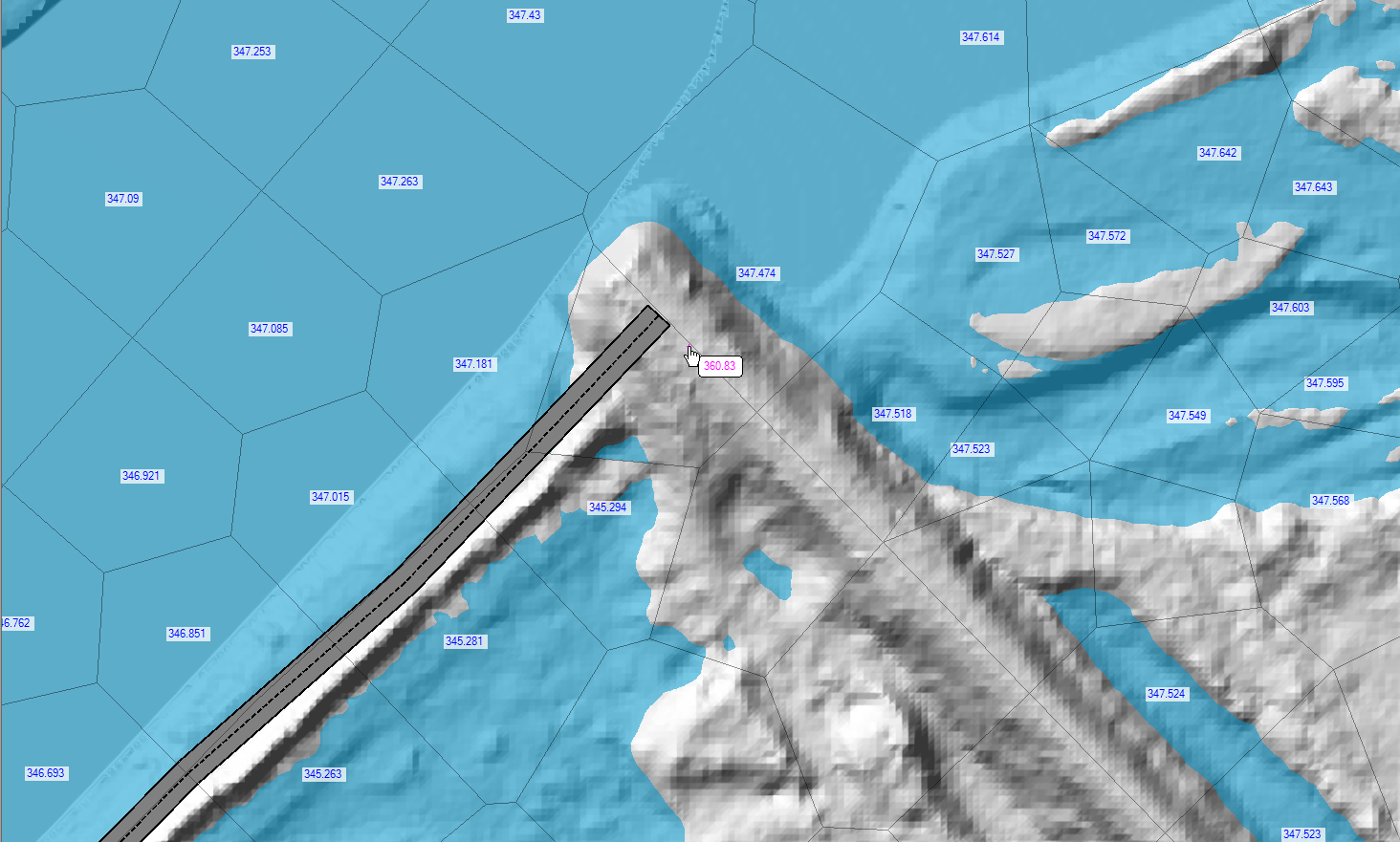
Draw Map Values
This plot option will label each 2D Cell with the value interpolated at the cell's computation point for particular layer. This is especially useful when considering water surface elevations and high ground.
In the example below, the water surface elevations are plotted to quickly see that the water surface is lower that the high ground elevation for the surrounding levee. This allows the modeler to more quickly identify a mesh (cell face) problems.
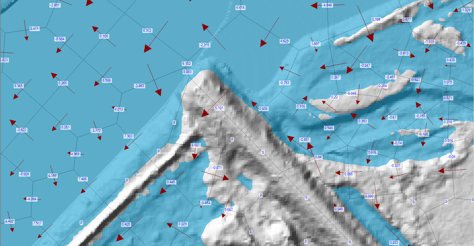
Draw Perpendicular Face Velocities
The option to draw perpendicular face velocities will show the modeler which cell faces have flow passing through them and label the magnitude of the velocity. Velocity vectors will be scaled base on magnitude to allow the modeler to more easily distinguish high and low flow locations. Keep in mind, this is only showing the velocity component perpendicular to the face; a fast flow that is mostly parallel to a given face will show very low values.
Face Low-Elevation Centroid
The location of the lowest point on a cell face can be displayed by turning on the Face Low-Elevation Centroid. The location does not show the exact low spot on the face, rather accumulates the lowest 5% of face elevations and computes the centroid. This will help the modeler identify low portions of the cell face and help explain water movement.
An example using the low face elevations is shown below.

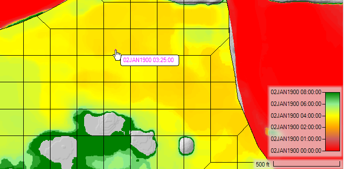
Display Arrival Times as Dates
The Arrival Time result map is computed either with hours or days from a simulation start time. Use this option if you would like to display the arrival date/time when hovering mouse cursor over the Arrival Time map. As shown in the example below, the map legend will also be shown using data/time.
Plot Model Boundary Deficiencies
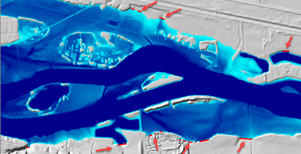
The Plot Model Boundary Deficiencies plot option is available to show the user where the inundation boundary is being limited by the model domain or the Edge Lines layer. This will occur where cross sections are not wide enough to capture the entire floodplain or the inundation occurs at the boundary of a 2D Flow Area. This tool can be helpful in model analysis and refinement.
The image below demonstrates a model deficiency in cross section layout.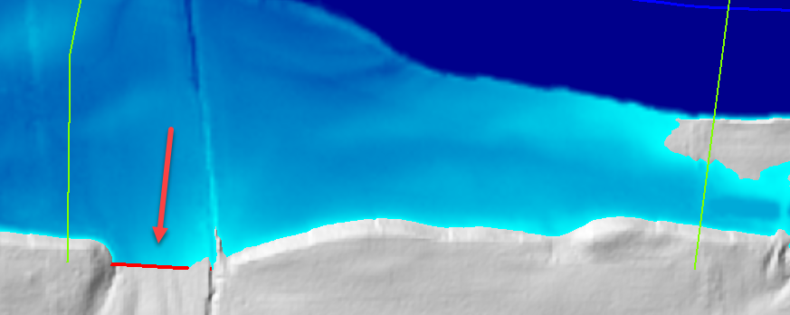
The example below shows several areas where a 2D Flow Area should be expanded to properly capture the floodplain.