Download PDF
Download page HOW TO Add Real-Time Gate Operation Capability to a ResSim Model.
HOW TO Add Real-Time Gate Operation Capability to a ResSim Model
Reservoir releases in ResSim can be limited by gate rating curves, but gate operation (i.e. user-control of gate settings) is not native to the ResSim user interface as of version 3.5. However, there is a modeling strategy that allows for real-time gate operations to be added to a ResSim model via "dummy" local flow timeseries and scripted rules. The Operation Support Interface (OSI) can then be used to set the gate opening at any timestep. If the alternative uses forecasted inflows, water managers can use the model to run what-if scenarios with different gate settings and identify the optimal gate setting schedule for the dam.
Step-by-step guide
The general workflow when adding real-time gate operation capability is to first create a "dummy" junction in the network that is connected to the upstream-most model element via a 0 flow diversion. Then add a local flow timeseries to the dummy junction for each gate to be operated. At each reservoir, add a scripted rule that uses pool elevation, tailwater elevation, and gate settings to compute a specified discharge. Then set up an OSI for each reservoir, adding each gate opening local flow timeseries as variables. These steps are described in more detail below using a fictional example of a reservoir with three, 12-foot wide lift gates.
Gate settings do not need to be added as a local inflow timeseries in all cases. Sometimes, gate settings can be included as a global variable or hard-coded directly into a scripted rule. However, gate settings must be included as local inflow timeseries if the user wishes to edit the gate settings in the OSI.
1. Add a dummy junction with a dummy diversion
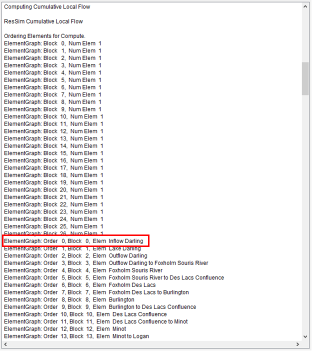
Add a junction to the network such that the new, "dummy" junction is the upstream-most element in the network. Being the upstream-most element is important because the junction needs to be computed before any of the reservoirs that use the gate setting timeseries. If there are multiple junctions or reservoirs that could be considered the most upstream element, and you do not know which element ResSim computes first, run a simulation and then open the compute report, as shown below.

In the compute report, scroll down to where it says "ElementGraph Order, Block 0." This is the first element ResSim calculates during the compute. In the example below, the "Inflow Darling" junction is the first element computed, so the dummy junction needs to be placed above the "Inflow Darling" junction.
The stream alignment may need to be edited in the Watershed Setup module to allow for the placement of a junction above the upstream-most element.
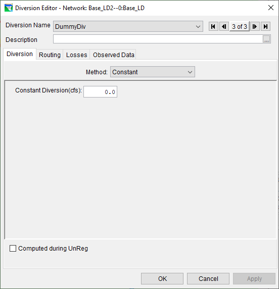
Once the dummy junction is created, a diversion needs to be created that connects the dummy junction to the upstream-most element. The diversion should be a constant, 0 cfs diversion, as shown below. This way, any amount of "inflow" can be added to the dummy junction, and the actual inflow to the model will not be affected. This is important because the gate setting timeseries are going to be added as local inflow timeseries, and we do not want them to actually contribute any inflow to the system.
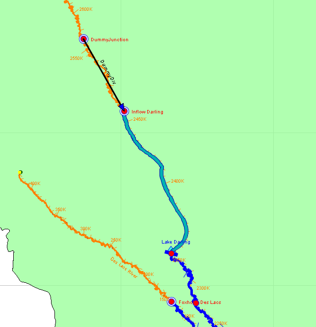
The final configuration of the dummy junction and dummy diversion is shown below.
2. Add gate settings as local inflow timeseries to the dummy junction
Each gate that is going to be operated needs to have its own gate setting timeseries. If a structure has many gates, and they are typically operated in groups, then a timeseries could be created for each group instead of each individual gate. Consider grouping gates if your ResSim model is complex and you would like to limit run times. The gate setting timeseries should be created in HEC-DSSVue with units of FLOW. Once created, they need to be added as local inflow timeseries to the dummy junction, as shown below. Once added to the junction, the dss files need to be linked in the alternative editor.

3. Add a scripted rule that computes discharge using the gate settings
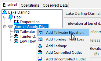
Now that the gate setting timeseries are in the model, we can use them in a scripted rule to compute discharge from the dam. In this example, discharge is dependent on pool elevation, tailwater elevation, and gate setting. Pool elevation is always a model timeseries, but tailwater elevation must be added to the dam in the physical data editor, as shown below. In most cases, adding tailwater in this way with a simple stage-discharge relationship is sufficient. However, if tailwater at your dam is dependent on some other variable, like backflow from a larger river directly downstream, a tailwater timeseries will need to be added to the model another way. Possible options could be a rating curve at another junction in the model, a global variable, or an extra computation within the scripted rule.
Once tailwater has been added to the model, the scripted rule can be defined. The example below shows a scripted rule that computes discharge through three, 12-foot lift gates (sometimes called slide gates). The rule defines a function within the initialization step called "liftGateCalc" that computes discharge through one, 12-foot wide lift gate using pool elevation, tailwater elevation, and gate opening. The function uses the weir equation if the gate is out of the water and the sluice gate equation if the gate is in the water. Each timestep during the compute, discharge through each gate is computed and then summed to get the total flow through the structure. Note the ruletype is set to SPEC, which forces the reservoir to release the computed discharge.
# required imports to create the OpValue return object.
from hec.rss.model import OpValue
from hec.rss.model import OpRule
from hec.script import Constants

#
# initialization function. optional.
#
# set up tables and other things that only need to be performed once during
# the compute.
#
# currentRule is the rule that holds this script
# network is the ResSim network
#
#
def initRuleScript(currentRule, network):

	# Put functions in a class so they can be retrieved in the main block
	class initFunctions:

		# Lift gate calc
		def liftGateCalc(self, poolElev, tailElev, gateOpening):

			# Assumed 0.65 for non-submerged flow coefficient (Cf)
			# Assumed 0.8 for submerged flow coefficient (Cs)
			# Assumed 3.2 for weir equation coefficient (C)
			Cf = 0.65
			Cs = 0.8
			C = 3.2
			g = 32.2
			width = 12
			crest = 1577

			# Compute head
			H = poolElev - crest
			Hb = tailElev - crest

			# Check for sluice vs. free weir flow condition
			if (crest + gateOpening) > poolElev and gateOpening > 0:

				# Weir flow
				# Compute discharge through the gate
				if poolElev < crest:
					# No flow
					Q = 0
				elif tailElev > poolElev:
					# No flow
					Q = 0
				elif tailElev < crest:
					# Free wier flow over crest
					Q = C*width*H**1.5
				else:
					# Villemonte flow
					Q = C*width*H**1.5*(1-(Hb/H)**1.5)**0.385
				return Q

			else:

				# Sluice gate flow
				# Compute submergence
				if tailElev == poolElev:
					sub = 1
				else:
					sub = (tailElev-crest)/(poolElev-crest)

				# Compute discharge through the gate
				if sub>= 1:
					# Backflow
					Q = 0
				elif sub < 0.67:
					# Free flowing sluice gate equation (RAS Ref Manual eq. 8-4)
					Q = Cf*width*gateOpening*(2*g*(poolElev-crest))**0.5
				elif sub >= 0.67 and sub <= 0.8:
					# Weighted avg of transition equation (RAS Ref Manual eq. 8-5) and fully submerged equation (RAS Ref Manual eq. 8-3)
					Q = Cf*width*gateOpening*(2*g*3*(poolElev-tailElev))**0.5*(1-((sub-0.67)/(0.8-0.67)))+Cs*width*gateOpening*(2*g*(poolElev-tailElev))**0.5*((sub-0.67)/(0.8-0.67))
				else:
					# Fully submerged equation (RAS Ref Manual eq. 8-3)
					Q = Cs*width*gateOpening*(2*g*(poolElev-tailElev))**0.5
				return Q

	# Initialize class
	functClass = initFunctions()
	# Store class in varaible
	currentRule.varPut('functClass',functClass)

	return Constants.TRUE

# runRuleScript() is the entry point that is called during the
# compute.
#
# currentRule is the rule that holds this script
# network is the ResSim network
# currentRuntimestep is the current Run Time Step
def runRuleScript(currentRule, network, currentRuntimestep):

	# Create new Operation Value (OpValue) to return
	opValue = OpValue()

	# Get inputs
	poolElev = network.getTimeSeries("Reservoir","Lake Darling", "Pool", "Elev").getPreviousValue(currentRuntimestep)
	tailElev = network.getTimeSeries("Reservoir","Lake Darling", "Dam at Souris River Tailwater", "Elev-TAILWATER").getPreviousValue(currentRuntimestep)
	liftGateOpening1 = network.findJunction("DummyJunction").getLocalFlowTimeSeries("LiftGate1").getCurrentValue(currentRuntimestep)
	liftGateOpening2 = network.findJunction("DummyJunction").getLocalFlowTimeSeries("LiftGate2").getCurrentValue(currentRuntimestep)
	liftGateOpening3 = network.findJunction("DummyJunction").getLocalFlowTimeSeries("LiftGate3").getCurrentValue(currentRuntimestep)

	# Get function class from init
	functClass = currentRule.varGet("functClass")

	# Compute discharge through each gate
	Q1 = functClass.liftGateCalc(poolElev, tailElev, liftGateOpening1)
	Q2 = functClass.liftGateCalc(poolElev, tailElev, liftGateOpening2)
	Q3 = functClass.liftGateCalc(poolElev, tailElev, liftGateOpening3)

	# Compute total discharge
	Q = Q1 + Q2 + Q3

	# set type and value for OpValue
	#  type is one of:
	#  OpRule.RULETYPE_MAX  - maximum flow
	#  OpRule.RULETYPE_MIN  - minimum flow
	#  OpRule.RULETYPE_SPEC - specified flow
	opValue.init(OpRule.RULETYPE_SPEC, Q)

	# return the Operation Value.
	# return "None" to have no effect on the compute
	return opValue
4. Add the gate setting local inflow timeseries to the OSI
At this point, the gate settings are being used in the ResSim model to compute discharge from the dam. However, the modeler needs to edit the gate setting timeseries in DSSVue and then rerun the extract in order to change the gate settings. To make editing gate settings and running what-if scenarios easier, the gate setting timeseries can be added to the OSI. The OSI can then be used to directly edit the gate settings, rerun the simulation, and view results all in one place.
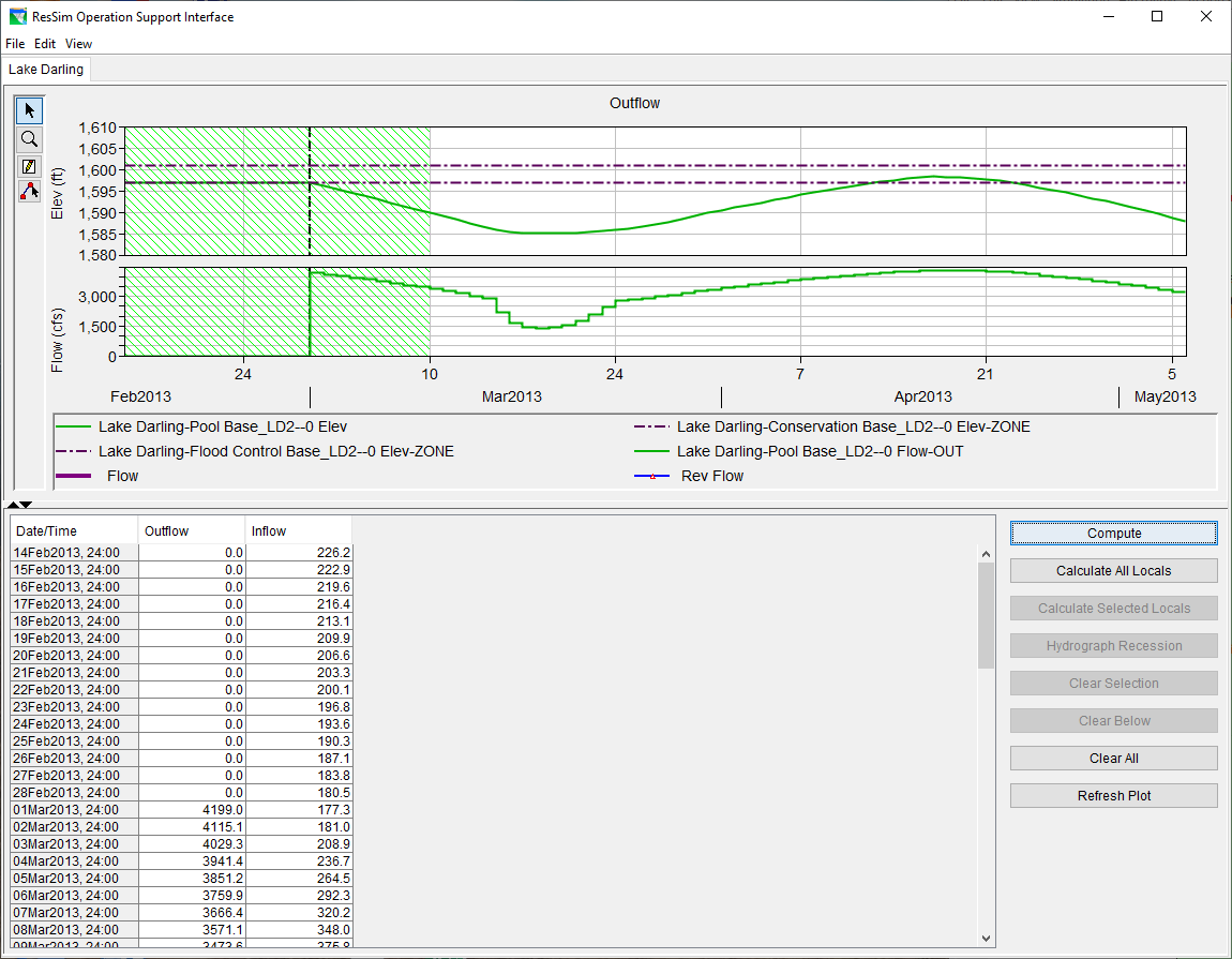
In the example below, an OSI has been set up for Lake Darling reservoir with two variables, Outflow and Inflow. The pool elevation, conservation zone elevation, and flood control zone elevation were added to the Outflow variable in a second viewport, as shown below.
To add one of the gate setting timeseries, add a variable via Edit>Add Variable in the OSI toolbar. Name the variable accordingly, then use the variable editor to select the corresponding local inflow to the dummy junction, as shown below. In the example below, the pool elevation, conservation zone elevation, and flood control zone elevation have been added to a second viewport so they will be plotted when the gate setting variable is selected.
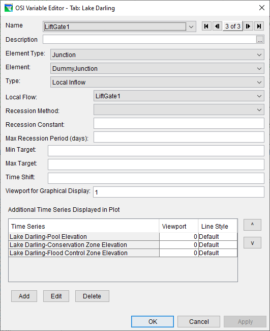
When adding Additional Timeseries Displayed in Plot to a variable, the user must select Apply before they can Add any timeseries.
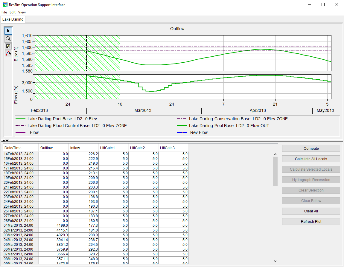
Repeat the previous step for each gate setting timeseries. Shown below is the example OSI with all three gate setting timeseries added.
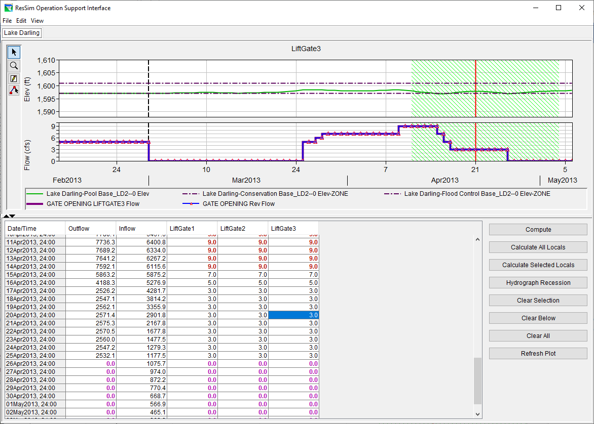
Now that the gate setting timeseries are added to the OSI, you can easily edit them, rerun the simulation, and view results. In the example above, the pool dropped far below its conservation elevation, and then rose above its conservation elevation later during the flood peak. This indicates the gates were open too far at the beginning of the simulation, and not far enough during the peak of the event. The screenshot below shows the gate settings edited such that the pool stays near its conservation elevation throughout the simulation.
The OSI must be saved, closed, and reopened before you can edit any of the timeseries.
Related articles
-
Page: